Radix Sort – Data Structures and Algorithms Tutorials
**Radix Sort** is a linear sorting algorithm that sorts elements by processing them digit by digit. It is an efficient sorting algorithm for integers or strings with fixed-size keys.
Rather than comparing elements directly, Radix Sort distributes the elements into buckets based on each digit’s value. By repeatedly sorting the elements by their significant digits, from the least significant to the most significant, Radix Sort achieves the final sorted order.
Radix Sort Algorithm
The key idea behind Radix Sort is to exploit the concept of place value. It assumes that sorting numbers digit by digit will eventually result in a fully sorted list. Radix Sort can be performed using different variations, such as Least Significant Digit (LSD) Radix Sort or Most Significant Digit (MSD) Radix Sort.
How does Radix Sort Algorithm work?
To perform radix sort on the array [170, 45, 75, 90, 802, 24, 2, 66], we follow these steps:
How does Radix Sort Algorithm work
Step 1 **Step 1:** Find the largest element in the array, which is 802. It has three digits, so we will iterate three times, once for each significant place.
**Step 2:** Sort the elements based on the unit place digits (X=0). We use a stable sorting technique, such as counting sort, to sort the digits at each significant place.
**Sorting based on the unit place:**
- Perform counting sort on the array based on the unit place digits.
- The sorted array based on the unit place is [170, 90, 802, 2, 24, 45, 75, 66].
How does Radix Sort Algorithm work
Step 2 **Step 3:** Sort the elements based on the tens place digits.
**Sorting based on the tens place:**
- Perform counting sort on the array based on the tens place digits.
- The sorted array based on the tens place is [802, 2, 24, 45, 66, 170, 75, 90].
How does Radix Sort Algorithm work
Step 3 **Step 4:** Sort the elements based on the hundreds place digits.
**Sorting based on the hundreds place:**
- Perform counting sort on the array based on the hundreds place digits.
- The sorted array based on the hundreds place is [2, 24, 45, 66, 75, 90, 170, 802].
How does Radix Sort Algorithm work
Step 4 **Step 5:** The array is now sorted in ascending order.
The final sorted array using radix sort is [2, 24, 45, 66, 75, 90, 170, 802].
How does Radix Sort Algorithm work
Step 5
Below is the implementation for the above illustrations:
// C++ implementation of Radix Sort

#include <iostream>

using namespace std;

// A utility function to get maximum
// value in arr[]
int getMax(int arr[], int n)
{
    int mx = arr[0];
    for (int i = 1; i < n; i++)
        if (arr[i] > mx)
            mx = arr[i];
    return mx;
}

// A function to do counting sort of arr[]
// according to the digit
// represented by exp.
void countSort(int arr[], int n, int exp)
{

    // Output array
    int output[n];
    int i, count[10] = { 0 };

    // Store count of occurrences
    // in count[]
    for (i = 0; i < n; i++)
        count[(arr[i] / exp) % 10]++;

    // Change count[i] so that count[i]
    // now contains actual position
    // of this digit in output[]
    for (i = 1; i < 10; i++)
        count[i] += count[i - 1];

    // Build the output array
    for (i = n - 1; i >= 0; i--) {
        output[count[(arr[i] / exp) % 10] - 1] = arr[i];
        count[(arr[i] / exp) % 10]--;
    }

    // Copy the output array to arr[],
    // so that arr[] now contains sorted
    // numbers according to current digit
    for (i = 0; i < n; i++)
        arr[i] = output[i];
}

// The main function to that sorts arr[]
// of size n using Radix Sort
void radixsort(int arr[], int n)
{

    // Find the maximum number to
    // know number of digits
    int m = getMax(arr, n);

    // Do counting sort for every digit.
    // Note that instead of passing digit
    // number, exp is passed. exp is 10^i
    // where i is current digit number
    for (int exp = 1; m / exp > 0; exp *= 10)
        countSort(arr, n, exp);
}

// A utility function to print an array
void print(int arr[], int n)
{
    for (int i = 0; i < n; i++)
        cout << arr[i] << " ";
}

// Driver Code
int main()
{
    int arr[] = { 170, 45, 75, 90, 802, 24, 2, 66 };
    int n = sizeof(arr) / sizeof(arr[0]);

    // Function Call
    radixsort(arr, n);
    print(arr, n);
    return 0;
}
// Radix sort Java implementation

import java.io.*;
import java.util.*;

class Radix {

    // A utility function to get maximum value in arr[]
    static int getMax(int arr[], int n)
    {
        int mx = arr[0];
        for (int i = 1; i < n; i++)
            if (arr[i] > mx)
                mx = arr[i];
        return mx;
    }

    // A function to do counting sort of arr[] according to
    // the digit represented by exp.
    static void countSort(int arr[], int n, int exp)
    {
        int output[] = new int[n]; // output array
        int i;
        int count[] = new int[10];
        Arrays.fill(count, 0);

        // Store count of occurrences in count[]
        for (i = 0; i < n; i++)
            count[(arr[i] / exp) % 10]++;

        // Change count[i] so that count[i] now contains
        // actual position of this digit in output[]
        for (i = 1; i < 10; i++)
            count[i] += count[i - 1];

        // Build the output array
        for (i = n - 1; i >= 0; i--) {
            output[count[(arr[i] / exp) % 10] - 1] = arr[i];
            count[(arr[i] / exp) % 10]--;
        }

        // Copy the output array to arr[], so that arr[] now
        // contains sorted numbers according to current
        // digit
        for (i = 0; i < n; i++)
            arr[i] = output[i];
    }

    // The main function to that sorts arr[] of
    // size n using Radix Sort
    static void radixsort(int arr[], int n)
    {
        // Find the maximum number to know number of digits
        int m = getMax(arr, n);

        // Do counting sort for every digit. Note that
        // instead of passing digit number, exp is passed.
        // exp is 10^i where i is current digit number
        for (int exp = 1; m / exp > 0; exp *= 10)
            countSort(arr, n, exp);
    }

    // A utility function to print an array
    static void print(int arr[], int n)
    {
        for (int i = 0; i < n; i++)
            System.out.print(arr[i] + " ");
    }

    // Main driver method
    public static void main(String[] args)
    {
        int arr[] = { 170, 45, 75, 90, 802, 24, 2, 66 };
        int n = arr.length;

        // Function Call
        radixsort(arr, n);
        print(arr, n);
    }
}
// Radix sort Dart implementation

/// A utility function to get the maximum value of a `List<int>` [array]
int getMax(List<int> array) {
  int max = array[0];

  for (final it in array) {
    if (it > max) {
      max = it;
    }
  }

  return max;
}

/// A function to do counting sort of `List<int>` [array] according to the
/// digit represented by [exp].
List<int> countSort(List<int> array, int exp) {
  final length = array.length;
  final outputArr = List.filled(length, 0);
  // A list where index represents the digit and value represents the count of
  // occurrences
  final digitsCount = List.filled(10, 0);

  // Store count of occurrences in digitsCount[]
  for (final item in array) {
    final digit = item ~/ exp % 10;
    digitsCount[digit]++;
  }

  // Change digitsCount[i] so that digitsCount[i] now contains actual position
  // of this digit in outputArr[]
  for (int i = 1; i < 10; i++) {
    digitsCount[i] += digitsCount[i - 1];
  }

  // Build the output array
  for (int i = length - 1; i >= 0; i--) {
    final item = array[i];
    final digit = item ~/ exp % 10;
    outputArr[digitsCount[digit] - 1] = item;
    digitsCount[digit]--;
  }

  return outputArr;
}

/// The main function to that sorts a `List<int>` [array] using Radix sort
List<int> radixSort(List<int> array) {
  // Find the maximum number to know number of digits
  final maxNumber = getMax(array);
  // Shallow copy of the input array
  final sortedArr = List.of(array);

  // Do counting sort for every digit. Note that instead of passing digit
  // number, exp is passed. exp is 10^i, where i is current digit number
  for (int exp = 1; maxNumber ~/ exp > 0; exp *= 10) {
    final sortedIteration = countSort(sortedArr, exp);
    sortedArr.clear();
    sortedArr.addAll(sortedIteration);
  }

  return sortedArr;
}

void main() {
  const array = [170, 45, 75, 90, 802, 24, 2, 66];

  final sortedArray = radixSort(array);

  print(sortedArray);
}

// This code is contributed by beeduhboodee
Output
2 24 45 66 75 90 170 802
[**Complexity Analysis of Radix Sort](https://www.geeksforgeeks.org/time-and-space-complexity-of-radix-sort-algorithm/):** ————————————————————————————————————————————–
**Time Complexity:**
- Radix sort is a non-comparative integer sorting algorithm that sorts data with integer keys by grouping the keys by the individual digits which share the same significant position and value. It has a time complexity of **O(d * (n + b))**, where d is the number of digits, n is the number of elements, and b is the base of the number system being used.
- In practical implementations, radix sort is often faster than other comparison-based sorting algorithms, such as quicksort or merge sort, for large datasets, especially when the keys have many digits. However, its time complexity grows linearly with the number of digits, and so it is not as efficient for small datasets.
**Auxiliary Space:**
- Radix sort also has a space complexity of **O(n + b),** where n is the number of elements and b is the base of the number system. This space complexity comes from the need to create buckets for each digit value and to copy the elements back to the original array after each digit has been sorted.
Frequently Asked Questions about RadixSort
**Q1. Is Radix Sort preferable to Comparison based sorting algorithms like Quick-Sort?**
If we have log2n bits for every digit, the running time of Radix appears to be better than Quick Sort for a wide range of input numbers. The constant factors hidden in asymptotic notation are higher for Radix Sort and Quick-Sort uses hardware caches more effectively. Also, Radix sort uses counting sort as a subroutine and counting sort takes extra space to sort numbers.
**Q2.** **What if the elements are in the** **range from 1 to n**2**?**
- The lower bound for the Comparison based sorting algorithm (Merge Sort, Heap Sort, Quick-Sort .. etc) is Ω(nLogn), i.e., they cannot do better than **nLogn**. Counting sort is a linear time sorting algorithm that sort in O(n+k) time when elements are in the range from 1 to k.
- We can’t use counting sort because counting sort will take O(n2) which is worse than comparison-based sorting algorithms. Can we sort such an array in linear time?
- **Radix Sort** is the answer. The idea of Radix Sort is to do digit-by-digit sorting starting from the least significant digit to the most significant digit. Radix sort uses counting sort as a subroutine to sort.
Bubble Sort – Data Structure and Algorithm Tutorials ====================================================
**Bubble Sort** is the simplest sorting algorithm that works by repeatedly swapping the adjacent elements if they are in the wrong order. This algorithm is not suitable for large data sets as its average and worst-case time complexity is quite high.
Bubble Sort Algorithm
In Bubble Sort algorithm,
- traverse from left and compare adjacent elements and the higher one is placed at right side.
- In this way, the largest element is moved to the rightmost end at first.
- This process is then continued to find the second largest and place it and so on until the data is sorted.
Recommended PracticeBubble SortTry It!How does Bubble Sort Work?
Let us understand the working of bubble sort with the help of the following illustration:
**Input:** arr[] = {6, 0, 3, 5}
**First Pass:**
The largest element is placed in its correct position, i.e., the end of the array.
Bubble Sort Algorithm : Placing the largest element at correct position
**Second Pass:**
Place the second largest element at correct position
Bubble Sort Algorithm : Placing the second largest element at correct position
**Third Pass:**
Place the remaining two elements at their correct positions.
Bubble Sort Algorithm : Placing the remaining elements at their correct positions
- **Total no. of passes:** n-1
- **Total no. of comparisons:** n*(n-1)/2
Implementation of Bubble Sort
Below is the implementation of the bubble sort. It can be optimized by stopping the algorithm if the inner loop didn’t cause any swap.
// Optimized implementation of Bubble sort
#include <bits/stdc++.h>
using namespace std;

// An optimized version of Bubble Sort
void bubbleSort(int arr[], int n)
{
    int i, j;
    bool swapped;
    for (i = 0; i < n - 1; i++) {
        swapped = false;
        for (j = 0; j < n - i - 1; j++) {
            if (arr[j] > arr[j + 1]) {
                swap(arr[j], arr[j + 1]);
                swapped = true;
            }
        }

        // If no two elements were swapped
        // by inner loop, then break
        if (swapped == false)
            break;
    }
}

// Function to print an array
void printArray(int arr[], int size)
{
    int i;
    for (i = 0; i < size; i++)
        cout << " " << arr[i];
}

// Driver program to test above functions
int main()
{
    int arr[] = { 64, 34, 25, 12, 22, 11, 90 };
    int N = sizeof(arr) / sizeof(arr[0]);
    bubbleSort(arr, N);
    cout << "Sorted array: \n";
    printArray(arr, N);
    return 0;
}
// This code is contributed by shivanisinghss2110
// Optimized java implementation of Bubble sort

import java.io.*;

class GFG {

    // An optimized version of Bubble Sort
    static void bubbleSort(int arr[], int n)
    {
        int i, j, temp;
        boolean swapped;
        for (i = 0; i < n - 1; i++) {
            swapped = false;
            for (j = 0; j < n - i - 1; j++) {
                if (arr[j] > arr[j + 1]) {

                    // Swap arr[j] and arr[j+1]
                    temp = arr[j];
                    arr[j] = arr[j + 1];
                    arr[j + 1] = temp;
                    swapped = true;
                }
            }

            // If no two elements were
            // swapped by inner loop, then break
            if (swapped == false)
                break;
        }
    }

    // Function to print an array
    static void printArray(int arr[], int size)
    {
        int i;
        for (i = 0; i < size; i++)
            System.out.print(arr[i] + " ");
        System.out.println();
    }

    // Driver program
    public static void main(String args[])
    {
        int arr[] = { 64, 34, 25, 12, 22, 11, 90 };
        int n = arr.length;
        bubbleSort(arr, n);
        System.out.println("Sorted array: ");
        printArray(arr, n);
    }
}

// This code is contributed
// by Nikita Tiwari.
Output
Sorted array:
 11 12 22 25 34 64 90
Complexity Analysis of Bubble Sort: ———————————————————————————————————————–
**Time Complexity:** O(N2)
**Auxiliary Space:** O(1)
**Advantages of Bubble Sort:**
- Bubble sort is easy to understand and implement.
- It does not require any additional memory space.
- It is a stable sorting algorithm, meaning that elements with the same key value maintain their relative order in the sorted output.
**Disadvantages of Bubble Sort:**
- Bubble sort has a time complexity of O(N2) which makes it very slow for large data sets.
- Bubble sort is a comparison-based sorting algorithm, which means that it requires a comparison operator to determine the relative order of elements in the input data set. It can limit the efficiency of the algorithm in certain cases.
Some FAQs related to Bubble Sort:
**What is the Boundary Case for Bubble sort?**
Bubble sort takes minimum time (Order of n) when elements are already sorted. Hence it is best to check if the array is already sorted or not beforehand, to avoid O(N2) time complexity.
Does sorting happen in place in Bubble sort?
Yes, Bubble sort performs the swapping of adjacent pairs without the use of any major data structure. Hence Bubble sort algorithm is an in-place algorithm.
Is the Bubble sort algorithm stable?
Yes, the bubble sort algorithm is stable.
Where is the Bubble sort algorithm used?
Due to its simplicity, bubble sort is often used to introduce the concept of a sorting algorithm. In computer graphics, it is popular for its capability to detect a tiny error (like a swap of just two elements) in almost-sorted arrays and fix it with just linear complexity (2n).
Example: It is used in a polygon filling algorithm, where bounding lines are sorted by their x coordinate at a specific scan line (a line parallel to the x-axis), and with incrementing y their order changes (two elements are swapped) only at intersections of two lines.
**Related Articles:**
- Recursive Bubble Sort
- Coding practice for sorting
- Quiz on Bubble Sort
- Complexity Analysis of Bubble Sort
Insertion Sort – Data Structure and Algorithm Tutorials =======================================================
**Insertion sort** is a simple sorting algorithm that works by iteratively inserting each element of an unsorted list into its correct position in a sorted portion of the list. It is a **stable sorting** algorithm, meaning that elements with equal values maintain their relative order in the sorted output.
**Insertion sort** is like sorting playing cards in your hands. You split the cards into two groups: the sorted cards and the unsorted cards. Then, you pick a card from the unsorted group and put it in the right place in the sorted group.
Insertion Sort Algorithm:
**Insertion sort** is a simple sorting algorithm that works by building a sorted array one element at a time. It is considered an “**in-place**” sorting algorithm, meaning it doesn’t require any additional memory space beyond the original array.
**Algorithm:**
To achieve insertion sort, follow these steps:
- We have to start with second element of the array as first element in the array is assumed to be sorted.
- Compare second element with the first element and check if the second element is smaller then swap them.
- Move to the third element and compare it with the second element, then the first element and swap as necessary to put it in the correct position among the first three elements.
- Continue this process, comparing each element with the ones before it and swapping as needed to place it in the correct position among the sorted elements.
- Repeat until the entire array is sorted.
Working of Insertion Sort Algorithm:
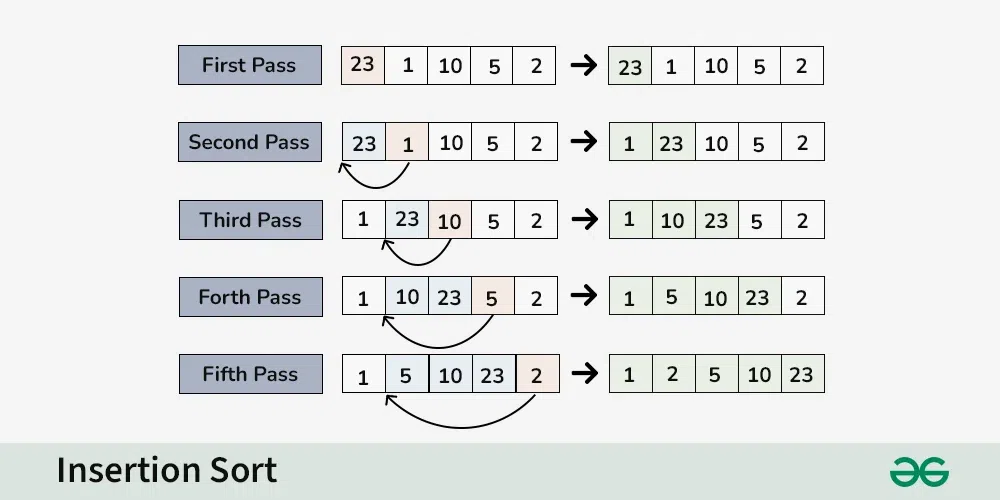
Consider an array having elements**: {23, 1, 10, 5, 2}**
**First Pass:**
- Current element is **23**
- The first element in the array is assumed to be sorted.
- The sorted part until **0th** index is : **[23]**
**Second Pass:**
- Compare **1** with **23** (current element with the sorted part).
- Since **1** is smaller, insert **1** before **23**.
- The sorted part until **1st** index is: **[1, 23]**
**Third Pass:**
- Compare **10** with **1** and **23** (current element with the sorted part).
- Since **10** is greater than **1** and smaller than **23, insert **10** between **1** and **23**.
- The sorted part until **2nd** index is: **[1, 10, 23]**
**Fourth Pass:**
- Compare **5** with **1, **10**, and **23** (current element with the sorted part).
- Since **5** is greater than **1** and smaller than **10, insert **5** between **1** and **10**.
- The sorted part until **3rd** index is**:** **[1, 5, 10, 23]**
**Fifth Pass:**
- Compare **2** with **1, 5, 10, and **23** (current element with the sorted part).
- Since **2** is greater than **1** and smaller than **5** insert **2** between **1** and **5**.
- The sorted part until **4th** index is: **[1, 2, 5, 10, 23]**
**Final Array:**
- The sorted array is: **[1, 2, 5, 10, 23]**
Recommended PracticeInsertion SortTry It!Implementation of Insertion Sort:
// C++ program for insertion sort

#include <bits/stdc++.h>
using namespace std;

// Function to sort an array using
// insertion sort
void insertionSort(int arr[], int n)
{
    int i, key, j;
    for (i = 1; i < n; i++) {
        key = arr[i];
        j = i - 1;

        // Move elements of arr[0..i-1],
        // that are greater than key,
        // to one position ahead of their
        // current position
        while (j >= 0 && arr[j] > key) {
            arr[j + 1] = arr[j];
            j = j - 1;
        }
        arr[j + 1] = key;
    }
}

// A utility function to print an array
// of size n
void printArray(int arr[], int n)
{
    int i;
    for (i = 0; i < n; i++)
        cout << arr[i] << " ";
    cout << endl;
}

// Driver code
int main()
{
    int arr[] = { 12, 11, 13, 5, 6 };
    int N = sizeof(arr) / sizeof(arr[0]);

    insertionSort(arr, N);
    printArray(arr, N);

    return 0;
}
// This is code is contributed by rathbhupendra
// Java program for implementation of Insertion Sort
public class InsertionSort {
    /*Function to sort array using insertion sort*/
    void sort(int arr[])
    {
        int n = arr.length;
        for (int i = 1; i < n; ++i) {
            int key = arr[i];
            int j = i - 1;

            /* Move elements of arr[0..i-1], that are
               greater than key, to one position ahead
               of their current position */
            while (j >= 0 && arr[j] > key) {
                arr[j + 1] = arr[j];
                j = j - 1;
            }
            arr[j + 1] = key;
        }
    }

    /* A utility function to print array of size n*/
    static void printArray(int arr[])
    {
        int n = arr.length;
        for (int i = 0; i < n; ++i)
            System.out.print(arr[i] + " ");

        System.out.println();
    }

    // Driver method
    public static void main(String args[])
    {
        int arr[] = { 12, 11, 13, 5, 6 };

        InsertionSort ob = new InsertionSort();
        ob.sort(arr);

        printArray(arr);
    }
};


/* This code is contributed by Rajat Mishra. */
Output
5 6 11 12 13
**Time Complexity:** O(N^2)
**Auxiliary Space:** O(1)
Complexity Analysis of Insertion Sort:
**Time Complexity of Insertion Sort**
- **Best case:** **O(n)**, If the list is already sorted, where n is the number of elements in the list.
- **Average case:** **O(n**2**)**, If the list is randomly ordered
- **Worst case:** **O(n**2**)**, If the list is in reverse order
Space Complexity **of Insertion Sort**
- **Auxiliary Space:** O(1), Insertion sort requires **O(1)** additional space, making it a space-efficient sorting algorithm.
Advantages **of Insertion Sort:**
- Simple and easy to implement.
- Stable sorting algorithm.
- Efficient for small lists and nearly sorted lists.
- Space-efficient.
Disadvantages **of Insertion Sort:**
- Inefficient for large lists.
- Not as efficient as other sorting algorithms (e.g., merge sort, quick sort) for most cases.
Applications **of Insertion Sort:**
Insertion sort is commonly used in situations where:
- The list is small or nearly sorted.
- Simplicity and stability are important.
Frequently Asked Questions on Insertion Sort
**Q1. What are the Boundary Cases of the Insertion Sort algorithm?**
Insertion sort takes the maximum time to sort if elements are sorted in reverse order. And it takes minimum time (Order of n) when elements are already sorted.
**Q2. What is the Algorithmic Paradigm of the Insertion Sort algorithm?**
The Insertion Sort algorithm follows an incremental approach.
**Q3. Is Insertion Sort an in-place sorting algorithm?**
Yes, insertion sort is an in-place sorting algorithm.
**Q4. Is Insertion Sort a stable algorithm?**
Yes, insertion sort is a stable sorting algorithm.
**Q5. When is the Insertion Sort algorithm used?**
Insertion sort is used when number of elements is small. It can also be useful when the input array is almost sorted, and only a few elements are misplaced in a complete big array.
Selection Sort – Data Structure and Algorithm Tutorials =======================================================
**Selection sort** is a simple and efficient sorting algorithm that works by repeatedly selecting the smallest (or largest) element from the unsorted portion of the list and moving it to the sorted portion of the list.
The algorithm repeatedly selects the smallest (or largest) element from the unsorted portion of the list and swaps it with the first element of the unsorted part. This process is repeated for the remaining unsorted portion until the entire list is sorted.
How does Selection Sort Algorithm work?
Lets consider the following array as an example: **arr[] = {64, 25, 12, 22, 11}**
**First pass:**
- For the first position in the sorted array, the whole array is traversed from index 0 to 4 sequentially. The first position where **64** is stored presently, after traversing whole array it is clear that **11** is the lowest value.
- Thus, replace 64 with 11. After one iteration **11**, which happens to be the least value in the array, tends to appear in the first position of the sorted list.
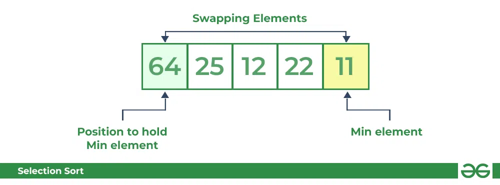Selection Sort Algorithm Swapping 1st element with the minimum in array **Second Pass:**
- For the second position, where 25 is present, again traverse the rest of the array in a sequential manner.
- After traversing, we found that **12** is the second lowest value in the array and it should appear at the second place in the array, thus swap these values.
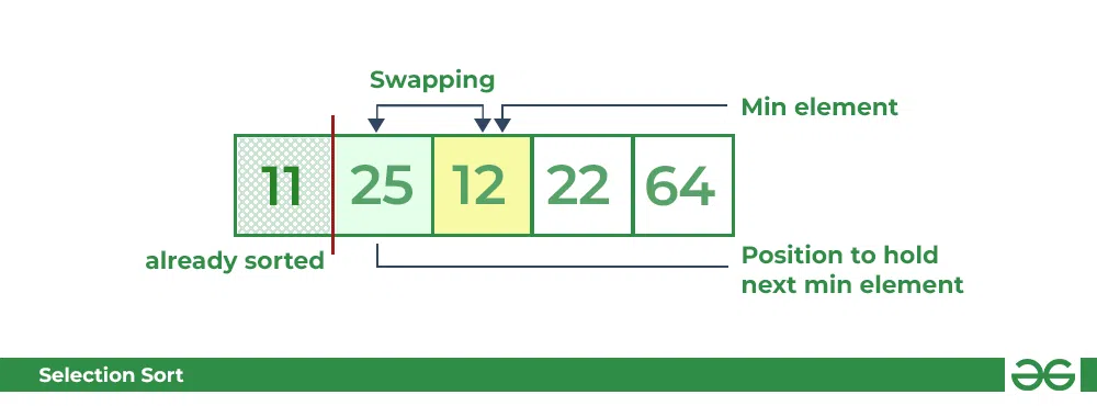Selection Sort Algorithm swapping i=1 with the next minimum element **Third Pass:**
- Now, for third place, where **25** is present again traverse the rest of the array and find the third least value present in the array.
- While traversing, **22** came out to be the third least value and it should appear at the third place in the array, thus swap **22** with element present at third position.
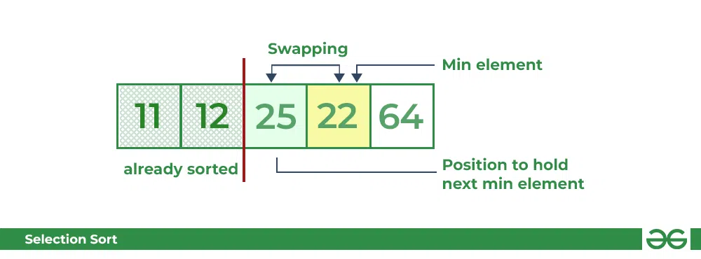Selection Sort Algorithm swapping i=2 with the next minimum element **Fourth pass:**
- Similarly, for fourth position traverse the rest of the array and find the fourth least element in the array
- As **25** is the 4th lowest value hence, it will place at the fourth position.
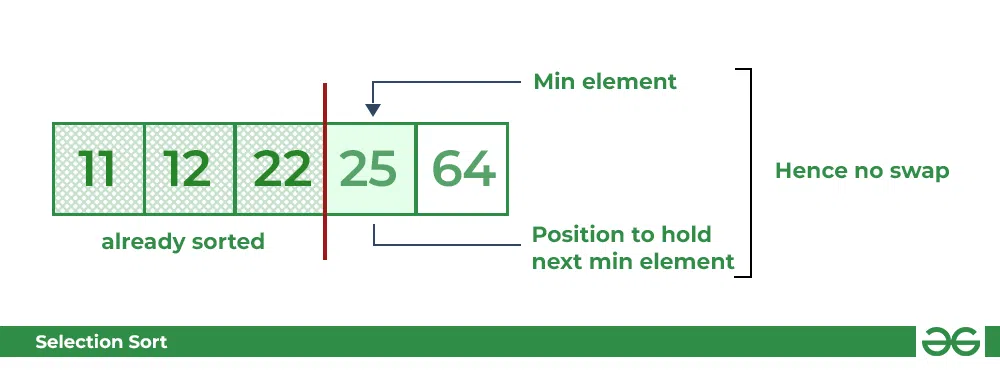Selection Sort Algorithm swapping i=3 with the next minimum element **Fifth Pass:**
- At last the largest value present in the array automatically get placed at the last position in the array
- The resulted array is the sorted array.
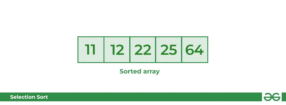Selection Sort Algorithm Required sorted array
Recommended PracticeSelection SortTry It! Below is the implementation of the above approach:
// C++ program for implementation of
// selection sort
#include <bits/stdc++.h>
using namespace std;

// Function for Selection sort
void selectionSort(int arr[], int n)
{
    int i, j, min_idx;

    // One by one move boundary of
    // unsorted subarray
    for (i = 0; i < n - 1; i++) {

        // Find the minimum element in
        // unsorted array
        min_idx = i;
        for (j = i + 1; j < n; j++) {
            if (arr[j] < arr[min_idx])
                min_idx = j;
        }

        // Swap the found minimum element
        // with the first element
        if (min_idx != i)
            swap(arr[min_idx], arr[i]);
    }
}

// Function to print an array
void printArray(int arr[], int size)
{
    int i;
    for (i = 0; i < size; i++) {
        cout << arr[i] << " ";
        cout << endl;
    }
}

// Driver program
int main()
{
    int arr[] = { 64, 25, 12, 22, 11 };
    int n = sizeof(arr) / sizeof(arr[0]);

    // Function Call
    selectionSort(arr, n);
    cout << "Sorted array: \n";
    printArray(arr, n);
    return 0;
}

// This is code is contributed by rathbhupendra
// Java program for implementation of Selection Sort
import java.io.*;
public class SelectionSort
{
    void sort(int arr[])
    {
        int n = arr.length;

        // One by one move boundary of unsorted subarray
        for (int i = 0; i < n-1; i++)
        {
            // Find the minimum element in unsorted array
            int min_idx = i;
            for (int j = i+1; j < n; j++)
                if (arr[j] < arr[min_idx])
                    min_idx = j;

            // Swap the found minimum element with the first
            // element
            int temp = arr[min_idx];
            arr[min_idx] = arr[i];
            arr[i] = temp;
        }
    }

    // Prints the array
    void printArray(int arr[])
    {
        int n = arr.length;
        for (int i=0; i<n; ++i)
            System.out.print(arr[i]+" ");
        System.out.println();
    }

    // Driver code to test above
    public static void main(String args[])
    {
        SelectionSort ob = new SelectionSort();
        int arr[] = {64,25,12,22,11};
        ob.sort(arr);
        System.out.println("Sorted array");
        ob.printArray(arr);
    }
}
/* This code is contributed by Rajat Mishra*/
Output
Sorted array:
11 12 22 25 64
Complexity Analysis of Selection Sort ————————————-
**Time Complexity:** The time complexity of Selection Sort is **O(N**2**)** as there are two nested loops:
- One loop to select an element of Array one by one = O(N)
- Another loop to compare that element with every other Array element = O(N)
- Therefore overall complexity = O(N) * O(N) = O(N*N) = O(N2)
**Auxiliary Space:** O(1) as the only extra memory used is for temporary variables while swapping two values in Array. The selection sort never makes more than O(N) swaps and can be useful when memory writing is costly.
Advantages of Selection Sort Algorithm
- Simple and easy to understand.
- Works well with small datasets.
**Disadvantages of the Selection Sort Algorithm**
- Selection sort has a time complexity of O(n^2) in the worst and average case.
- Does not work well on large datasets.
- Does not preserve the relative order of items with equal keys which means it is not stable.
Frequently Asked Questions on Selection Sort
**Q1. Is Selection Sort Algorithm stable?**
The default implementation of the Selection Sort Algorithm is **not stable**. However, it can be made stable. Please see the stable Selection Sort for details.
**Q2. Is Selection Sort Algorithm in-place?**
Yes, Selection Sort Algorithm is an in-place algorithm, as it does not require extra space.
QuickSort – Data Structure and Algorithm Tutorials ==================================================
**QuickSort** is a sorting algorithm based on the Divide and Conquer algorithm that picks an element as a pivot and partitions the given array around the picked pivot by placing the pivot in its correct position in the sorted array.
How does QuickSort work?
The key process in **quickSort** is a **partition()**. The target of partitions is to place the pivot (any element can be chosen to be a pivot) at its correct position in the sorted array and put all smaller elements to the left of the pivot, and all greater elements to the right of the pivot.
Partition is done recursively on each side of the pivot after the pivot is placed in its correct position and this finally sorts the array.
How Quicksort works
Recommended PracticeQuick SortTry It!### Choice of Pivot:
There are many different choices for picking pivots.
- Always pick the first element as a pivot.
- Always pick the last element as a pivot (implemented below)
- Pick a random element as a pivot.
- Pick the middle as the pivot.
Partition Algorithm:
The logic is simple, we start from the leftmost element and keep track of the index of smaller (or equal) elements as **i**. While traversing, if we find a smaller element, we swap the current element with arr[i]. Otherwise, we ignore the current element.
Let us understand the working of partition and the Quick Sort algorithm with the help of the following example:
Consider: arr[] = {10, 80, 30, 90, 40}.
- Compare 10 with the pivot and as it is less than pivot arrange it accrodingly.
Partition in QuickSort: Compare pivot with 10
- Compare 80 with the pivot. It is greater than pivot.
Partition in QuickSort: Compare pivot with 80
- Compare 30 with pivot. It is less than pivot so arrange it accordingly.
Partition in QuickSort: Compare pivot with 30
- Compare 90 with the pivot. It is greater than the pivot.
Partition in QuickSort: Compare pivot with 90
- Arrange the pivot in its correct position.
Partition in QuickSort: Place pivot in its correct position
Illustration of Quicksort:
As the partition process is done recursively, it keeps on putting the pivot in its actual position in the sorted array. Repeatedly putting pivots in their actual position makes the array sorted.
Follow the below images to understand how the recursive implementation of the partition algorithm helps to sort the array.
- Initial partition on the main array:
Quicksort: Performing the partition
- Partitioning of the subarrays:
Quicksort: Performing the partition
Code implementation of the Quick Sort:
#include <bits/stdc++.h>
using namespace std;

int partition(int arr[],int low,int high)
{
  //choose the pivot

  int pivot=arr[high];
  //Index of smaller element and Indicate
  //the right position of pivot found so far
  int i=(low-1);

  for(int j=low;j<=high;j++)
  {
    //If current element is smaller than the pivot
    if(arr[j]<pivot)
    {
      //Increment index of smaller element
      i++;
      swap(arr[i],arr[j]);
    }
  }
  swap(arr[i+1],arr[high]);
  return (i+1);
}

// The Quicksort function Implement

void quickSort(int arr[],int low,int high)
{
  // when low is less than high
  if(low<high)
  {
    // pi is the partition return index of pivot

    int pi=partition(arr,low,high);

    //Recursion Call
    //smaller element than pivot goes left and
    //higher element goes right
    quickSort(arr,low,pi-1);
    quickSort(arr,pi+1,high);
  }
}


int main() {
  int arr[]={10,7,8,9,1,5};
  int n=sizeof(arr)/sizeof(arr[0]);
  // Function call
  quickSort(arr,0,n-1);
  //Print the sorted array
  cout<<"Sorted Array\n";
  for(int i=0;i<n;i++)
  {
    cout<<arr[i]<<" ";
  }
  return 0;
}
// This Code is Contributed By Diwakar Jha
// Java implementation of QuickSort
import java.io.*;

class GFG {

    // A utility function to swap two elements
    static void swap(int[] arr, int i, int j)
    {
        int temp = arr[i];
        arr[i] = arr[j];
        arr[j] = temp;
    }

    // This function takes last element as pivot,
    // places the pivot element at its correct position
    // in sorted array, and places all smaller to left
    // of pivot and all greater elements to right of pivot
    static int partition(int[] arr, int low, int high)
    {
        // Choosing the pivot
        int pivot = arr[high];

        // Index of smaller element and indicates
        // the right position of pivot found so far
        int i = (low - 1);

        for (int j = low; j <= high - 1; j++) {

            // If current element is smaller than the pivot
            if (arr[j] < pivot) {

                // Increment index of smaller element
                i++;
                swap(arr, i, j);
            }
        }
        swap(arr, i + 1, high);
        return (i + 1);
    }

    // The main function that implements QuickSort
    // arr[] --> Array to be sorted,
    // low --> Starting index,
    // high --> Ending index
    static void quickSort(int[] arr, int low, int high)
    {
        if (low < high) {

            // pi is partitioning index, arr[p]
            // is now at right place
            int pi = partition(arr, low, high);

            // Separately sort elements before
            // partition and after partition
            quickSort(arr, low, pi - 1);
            quickSort(arr, pi + 1, high);
        }
    }
    // To print sorted array
    public static void printArr(int[] arr)
    {
        for (int i = 0; i < arr.length; i++) {
            System.out.print(arr[i] + " ");
        }
    }

    // Driver Code
    public static void main(String[] args)
    {
        int[] arr = { 10, 7, 8, 9, 1, 5 };
        int N = arr.length;

        // Function call
        quickSort(arr, 0, N - 1);
        System.out.println("Sorted array:");
        printArr(arr);
    }
}

// This code is contributed by Ayush Choudhary
// Improved by Ajay Virmoti
Output
Sorted Array
1 5 7 8 9 10
Complexity Analysis of Quick Sort: ———————————————————————————————————————
**Time Complexity:**
- **Best Case**: Ω (N log (N))
The best-case scenario for quicksort occur when the pivot chosen at the each step divides the array into roughly equal halves.
In this case, the algorithm will make balanced partitions, leading to efficient Sorting. - **Average Case: θ ( N log (N))**
Quicksort’s average-case performance is usually very good in practice, making it one of the fastest sorting Algorithm. - **Worst Case: O(N2)**
The worst-case Scenario for Quicksort occur when the pivot at each step consistently results in highly unbalanced partitions. When the array is already sorted and the pivot is always chosen as the smallest or largest element. To mitigate the worst-case Scenario, various techniques are used such as choosing a good pivot (e.g., median of three) and using Randomized algorithm (Randomized Quicksort ) to shuffle the element before sorting. - **Auxiliary Space:** O(1), if we don’t consider the recursive stack space. If we consider the recursive stack space then, in the worst case quicksort could make O(N).
**Advantages of Quick Sort:**
- It is a divide-and-conquer algorithm that makes it easier to solve problems.
- It is efficient on large data sets.
- It has a low overhead, as it only requires a small amount of memory to function.
Disadvantages of Quick Sort:
- It has a worst-case time complexity of O(N2), which occurs when the pivot is chosen poorly.
- It is not a good choice for small data sets.
- It is not a stable sort, meaning that if two elements have the same key, their relative order will not be preserved in the sorted output in case of quick sort, because here we are swapping elements according to the pivot’s position (without considering their original positions).
Time and Space Complexity Analysis of Quick Sort
Merge Sort – Data Structure and Algorithms Tutorials ====================================================
**Merge sort** is a sorting algorithm that follows the **divide-and-conquer** approach. It works by recursively dividing the input array into smaller subarrays and sorting those subarrays then merging them back together to obtain the sorted array.
In simple terms, we can say that the process of **merge sort** is to divide the array into two halves, sort each half, and then merge the sorted halves back together. This process is repeated until the entire array is sorted.
.png) Merge Sort Algorithm
Merge Sort Algorithm
How does Merge Sort work?
Merge sort is a popular sorting algorithm known for its efficiency and stability. It follows the **divide-and-conquer** approach to sort a given array of elements.
Here’s a step-by-step explanation of how merge sort works:
- **Divide:** Divide the list or array recursively into two halves until it can no more be divided.
- **Conquer:** Each subarray is sorted individually using the merge sort algorithm.
- **Merge:** The sorted subarrays are merged back together in sorted order. The process continues until all elements from both subarrays have been merged.
Illustration of Merge Sort:
Let’s sort the array or list **[38, 27, 43, 10]** using Merge Sort
Let’s look at the working of above example:
**Divide:**
- **[38, 27, 43, 10]** is divided into **[38, 27] and **[43, 10]**.
- **[38, 27]** is divided into **[38]** and **[27]**.
- **[43, 10]** is divided into **[43]** and **[10]**.
**Conquer:**
- **[38]** is already sorted.
- **[27]** is already sorted.
- **[43]** is already sorted.
- **[10]** is already sorted.
**Merge:**
- Merge **[38]** and **[27]** to get **[27, 38]**.
- Merge **[43]** and **[10]** to get **[10,43]**.
- Merge **[27, 38]** and **[10,43]** to get the final sorted list **[10, 27, 38, 43]**
Therefore, the sorted list is **[10, 27, 38, 43]**.
Recommended PracticeMerge SortTry It!Implementation of Merge Sort:
// C++ program for Merge Sort
#include <bits/stdc++.h>
using namespace std;

// Merges two subarrays of array[].
// First subarray is arr[begin..mid]
// Second subarray is arr[mid+1..end]
void merge(int array[], int const left, int const mid,
           int const right)
{
    int const subArrayOne = mid - left + 1;
    int const subArrayTwo = right - mid;

    // Create temp arrays
    auto *leftArray = new int[subArrayOne],
         *rightArray = new int[subArrayTwo];

    // Copy data to temp arrays leftArray[] and rightArray[]
    for (auto i = 0; i < subArrayOne; i++)
        leftArray[i] = array[left + i];
    for (auto j = 0; j < subArrayTwo; j++)
        rightArray[j] = array[mid + 1 + j];

    auto indexOfSubArrayOne = 0, indexOfSubArrayTwo = 0;
    int indexOfMergedArray = left;

    // Merge the temp arrays back into array[left..right]
    while (indexOfSubArrayOne < subArrayOne
           && indexOfSubArrayTwo < subArrayTwo) {
        if (leftArray[indexOfSubArrayOne]
            <= rightArray[indexOfSubArrayTwo]) {
            array[indexOfMergedArray]
                = leftArray[indexOfSubArrayOne];
            indexOfSubArrayOne++;
        }
        else {
            array[indexOfMergedArray]
                = rightArray[indexOfSubArrayTwo];
            indexOfSubArrayTwo++;
        }
        indexOfMergedArray++;
    }

    // Copy the remaining elements of
    // left[], if there are any
    while (indexOfSubArrayOne < subArrayOne) {
        array[indexOfMergedArray]
            = leftArray[indexOfSubArrayOne];
        indexOfSubArrayOne++;
        indexOfMergedArray++;
    }

    // Copy the remaining elements of
    // right[], if there are any
    while (indexOfSubArrayTwo < subArrayTwo) {
        array[indexOfMergedArray]
            = rightArray[indexOfSubArrayTwo];
        indexOfSubArrayTwo++;
        indexOfMergedArray++;
    }
    delete[] leftArray;
    delete[] rightArray;
}

// begin is for left index and end is right index
// of the sub-array of arr to be sorted
void mergeSort(int array[], int const begin, int const end)
{
    if (begin >= end)
        return;

    int mid = begin + (end - begin) / 2;
    mergeSort(array, begin, mid);
    mergeSort(array, mid + 1, end);
    merge(array, begin, mid, end);
}

// UTILITY FUNCTIONS
// Function to print an array
void printArray(int A[], int size)
{
    for (int i = 0; i < size; i++)
        cout << A[i] << " ";
    cout << endl;
}

// Driver code
int main()
{
    int arr[] = { 12, 11, 13, 5, 6, 7 };
    int arr_size = sizeof(arr) / sizeof(arr[0]);

    cout << "Given array is \n";
    printArray(arr, arr_size);

    mergeSort(arr, 0, arr_size - 1);

    cout << "\nSorted array is \n";
    printArray(arr, arr_size);
    return 0;
}

// This code is contributed by Mayank Tyagi
// This code was revised by Joshua Estes
// Java program for Merge Sort
import java.io.*;

class MergeSort {

    // Merges two subarrays of arr[].
    // First subarray is arr[l..m]
    // Second subarray is arr[m+1..r]
    void merge(int arr[], int l, int m, int r)
    {
        // Find sizes of two subarrays to be merged
        int n1 = m - l + 1;
        int n2 = r - m;

        // Create temp arrays
        int L[] = new int[n1];
        int R[] = new int[n2];

        // Copy data to temp arrays
        for (int i = 0; i < n1; ++i)
            L[i] = arr[l + i];
        for (int j = 0; j < n2; ++j)
            R[j] = arr[m + 1 + j];

        // Merge the temp arrays

        // Initial indices of first and second subarrays
        int i = 0, j = 0;

        // Initial index of merged subarray array
        int k = l;
        while (i < n1 && j < n2) {
            if (L[i] <= R[j]) {
                arr[k] = L[i];
                i++;
            }
            else {
                arr[k] = R[j];
                j++;
            }
            k++;
        }

        // Copy remaining elements of L[] if any
        while (i < n1) {
            arr[k] = L[i];
            i++;
            k++;
        }

        // Copy remaining elements of R[] if any
        while (j < n2) {
            arr[k] = R[j];
            j++;
            k++;
        }
    }

    // Main function that sorts arr[l..r] using
    // merge()
    void sort(int arr[], int l, int r)
    {
        if (l < r) {

            // Find the middle point
            int m = l + (r - l) / 2;

            // Sort first and second halves
            sort(arr, l, m);
            sort(arr, m + 1, r);

            // Merge the sorted halves
            merge(arr, l, m, r);
        }
    }

    // A utility function to print array of size n
    static void printArray(int arr[])
    {
        int n = arr.length;
        for (int i = 0; i < n; ++i)
            System.out.print(arr[i] + " ");
        System.out.println();
    }

    // Driver code
    public static void main(String args[])
    {
        int arr[] = { 12, 11, 13, 5, 6, 7 };

        System.out.println("Given array is");
        printArray(arr);

        MergeSort ob = new MergeSort();
        ob.sort(arr, 0, arr.length - 1);

        System.out.println("\nSorted array is");
        printArray(arr);
    }
}
/* This code is contributed by Rajat Mishra */
Output
Given array is
12 11 13 5 6 7

Sorted array is
5 6 7 11 12 13
**Complexity Analysis of Merge Sort:** ——————————————
**Time Complexity:**
- **Best Case:** O(n log n), When the array is already sorted or nearly sorted.
- **Average Case:** O(n log n), When the array is randomly ordered.
- **Worst Case:** O(n log n), When the array is sorted in reverse order.
**Space Complexity:** O(n), Additional space is required for the temporary array used during merging.
**Advantages of Merge Sort:**
- **Stability**: Merge sort is a stable sorting algorithm, which means it maintains the relative order of equal elements in the input array.
- **Guaranteed worst-case performance:** Merge sort has a worst-case time complexity of **O(N logN)**, which means it performs well even on large datasets.
- **Simple to implement:** The divide-and-conquer approach is straightforward.
**Disadvantage of Merge Sort:**
- **Space complexity:** Merge sort requires additional memory to store the merged sub-arrays during the sorting process.
- **Not in-place:** Merge sort is not an in-place sorting algorithm, which means it requires additional memory to store the sorted data. This can be a disadvantage in applications where memory usage is a concern.
Applications of Merge Sort:
- Sorting large datasets
- External sorting (when the dataset is too large to fit in memory)
- Inversion counting (counting the number of inversions in an array)
- Finding the median of an array
**Quick Links:**
- Recent Articles on Merge Sort
- Top Sorting Interview Questions and Problems
- Practice problems on Sorting algorithm
- Quiz on Merge Sort
Heap Sort – Data Structures and Algorithms Tutorials ====================================================
**Heap sort** is a comparison-based sorting technique based on Binary Heap data structure. It is similar to the selection sort where we first find the minimum element and place the minimum element at the beginning. Repeat the same process for the remaining elements.
Heap Sort Algorithm
To solve the problem follow the below idea:
First convert the array into heap data structure using heapify, then one by one delete the root node of the Max-heap and replace it with the last node in the heap and then heapify the root of the heap. Repeat this process until size of heap is greater than 1.
- Build a heap from the given input array.
- Repeat the following steps until the heap contains only one element:
- Swap the root element of the heap (which is the largest element) with the last element of the heap.
- Remove the last element of the heap (which is now in the correct position).
- Heapify the remaining elements of the heap.
- The sorted array is obtained by reversing the order of the elements in the input array.
Recommended Problem Please solve it on PRACTICE first, before moving on to the solution Solve Problem **Detailed Working of Heap Sort**
To understand heap sort more clearly, let’s take an unsorted array and try to sort it using heap sort.
Consider the array: arr[] = {4, 10, 3, 5, 1}.**Build Complete Binary Tree:** Build a complete binary tree from the array.
.webp)Heap sort algorithm Build Complete Binary Tree **Transform into max heap:** After that, the task is to construct a tree from that unsorted array and try to convert it into max heap.
- To transform a heap into a max-heap, the parent node should always be greater than or equal to the child nodes
- Here, in this example, as the parent node **4** is smaller than the child node **10,** thus, swap them to build a max-heap.
- Now, **4** as a parent is smaller than the child **5**, thus swap both of these again and the resulted heap and array should be like this:
.webp)Heap sort algorithm Max Heapify constructed binary tree **Perform heap sort:** Remove the maximum element in each step (i.e., move it to the end position and remove that) and then consider the remaining elements and transform it into a max heap.
- Delete the root element **(10)** from the max heap. In order to delete this node, try to swap it with the last node, i.e. **(1).** After removing the root element, again heapify it to convert it into max heap.
- Resulted heap and array should look like this:
.webp)Heap sort algorithm Remove maximum from root and max heapify
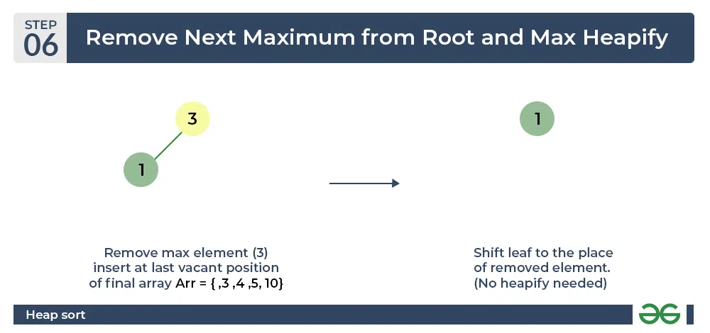
- Repeat the above steps and it will look like the following:
.webp)Heap sort algorithm Remove next maximum from root nad max heapify
- Now remove the root (i.e. 3) again and perform heapify.
Heap sort algorithm Repeat previous step
- Now when the root is removed once again it is sorted. and the sorted array will be like **arr[] = {1, 3, 4, 5, 10}**.
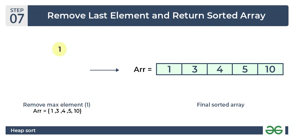Heap sort algorithm Final sorted array
Implementation of Heap Sort
// C++ program for implementation of Heap Sort

#include <iostream>
using namespace std;

// To heapify a subtree rooted with node i
// which is an index in arr[].
// n is size of heap
void heapify(int arr[], int N, int i)
{

    // Initialize largest as root
    int largest = i;

    // left = 2*i + 1
    int l = 2 * i + 1;

    // right = 2*i + 2
    int r = 2 * i + 2;

    // If left child is larger than root
    if (l < N && arr[l] > arr[largest])
        largest = l;

    // If right child is larger than largest
    // so far
    if (r < N && arr[r] > arr[largest])
        largest = r;

    // If largest is not root
    if (largest != i) {
        swap(arr[i], arr[largest]);

        // Recursively heapify the affected
        // sub-tree
        heapify(arr, N, largest);
    }
}

// Main function to do heap sort
void heapSort(int arr[], int N)
{

    // Build heap (rearrange array)
    for (int i = N / 2 - 1; i >= 0; i--)
        heapify(arr, N, i);

    // One by one extract an element
    // from heap
    for (int i = N - 1; i > 0; i--) {

        // Move current root to end
        swap(arr[0], arr[i]);

        // call max heapify on the reduced heap
        heapify(arr, i, 0);
    }
}

// A utility function to print array of size n
void printArray(int arr[], int N)
{
    for (int i = 0; i < N; ++i)
        cout << arr[i] << " ";
    cout << "\n";
}

// Driver's code
int main()
{
    int arr[] = { 12, 11, 13, 5, 6, 7 };
    int N = sizeof(arr) / sizeof(arr[0]);

    // Function call
    heapSort(arr, N);

    cout << "Sorted array is \n";
    printArray(arr, N);
}
// Java program for implementation of Heap Sort

public class HeapSort {
    public void sort(int arr[])
    {
        int N = arr.length;

        // Build heap (rearrange array)
        for (int i = N / 2 - 1; i >= 0; i--)
            heapify(arr, N, i);

        // One by one extract an element from heap
        for (int i = N - 1; i > 0; i--) {
            // Move current root to end
            int temp = arr[0];
            arr[0] = arr[i];
            arr[i] = temp;

            // call max heapify on the reduced heap
            heapify(arr, i, 0);
        }
    }

    // To heapify a subtree rooted with node i which is
    // an index in arr[]. n is size of heap
    void heapify(int arr[], int N, int i)
    {
        int largest = i; // Initialize largest as root
        int l = 2 * i + 1; // left = 2*i + 1
        int r = 2 * i + 2; // right = 2*i + 2

        // If left child is larger than root
        if (l < N && arr[l] > arr[largest])
            largest = l;

        // If right child is larger than largest so far
        if (r < N && arr[r] > arr[largest])
            largest = r;

        // If largest is not root
        if (largest != i) {
            int swap = arr[i];
            arr[i] = arr[largest];
            arr[largest] = swap;

            // Recursively heapify the affected sub-tree
            heapify(arr, N, largest);
        }
    }

    /* A utility function to print array of size n */
    static void printArray(int arr[])
    {
        int N = arr.length;

        for (int i = 0; i < N; ++i)
            System.out.print(arr[i] + " ");
        System.out.println();
    }

    // Driver's code
    public static void main(String args[])
    {
        int arr[] = { 12, 11, 13, 5, 6, 7 };
        int N = arr.length;

        // Function call
        HeapSort ob = new HeapSort();
        ob.sort(arr);

        System.out.println("Sorted array is");
        printArray(arr);
    }
}
Output
Sorted array is
5 6 7 11 12 13
Complexity Analysis of **Heap Sort** —————————————-
**Time Complexity:** O(N log N)
**Auxiliary Space:** O(log n), due to the recursive call stack. However, auxiliary space can be O(1) for iterative implementation.
**Important points about Heap Sort:**
- Heap sort is an in-place algorithm.
- Its typical implementation is not stable but can be made stable (See this)
- Typically 2-3 times slower than well-implemented QuickSort. The reason for slowness is a lack of locality of reference.
**Advantages of Heap Sort:**
- **Efficient Time Complexity:** Heap Sort has a time complexity of O(n log n) in all cases. This makes it efficient for sorting large datasets. The **log n** factor comes from the height of the binary heap, and it ensures that the algorithm maintains good performance even with a large number of elements.
- **Memory Usage –** Memory usage can be minimal (by writing an iterative heapify() instead of a recursive one). So apart from what is necessary to hold the initial list of items to be sorted, it needs no additional memory space to work
- **Simplicity –** It is simpler to understand than other equally efficient sorting algorithms because it does not use advanced computer science concepts such as recursion.
Disadvantages of Heap Sort:
- **Costly**: Heap sort is costly as the constants are higher compared to merge sort even if the time complexity is O(n Log n) for both.
- **Unstable**: Heap sort is unstable. It might rearrange the relative order.
- **Efficient:** Heap Sort is not very efficient when working with highly complex data.
Frequently Asked Questions Related to Heap Sort
**Q1. What are the two phases of Heap Sort?**
The heap sort algorithm consists of two phases. In the first phase, the array is converted into a max heap. And in the second phase, the highest element is removed (i.e., the one at the tree root) and the remaining elements are used to create a new max heap.
**Q2. Why Heap Sort is not stable?**
The heap sort algorithm is not a stable algorithm because we swap arr[i] with arr[0] in heapSort() which might change the relative ordering of the equivalent keys.
**Q3. Is Heap Sort an example of the “Divide and Conquer” algorithm?**
Heap sort is **NOT** at all a Divide and Conquer algorithm. It uses a heap data structure to efficiently sort its element and not a “divide and conquer approach” to sort the elements.
**Q4. Which sorting algorithm is better – Heap sort or Merge Sort?**
The answer lies in the comparison of their time complexity and space requirements. The Merge sort is slightly faster than the Heap sort. But on the other hand merge sort takes extra memory. Depending on the requirement, one should choose which one to use.
**Q5. Why is Heap sort better than Selection sort?**
Heap sort is similar to selection sort, but with a better way to get the maximum element. It takes advantage of the heap data structure to get the maximum element in constant time