Introduction to Graphs – Data Structure and Algorithm Tutorials
Graph data structures are a powerful tool for representing and analyzing complex relationships between objects or entities. They are particularly useful in fields such as social network analysis, recommendation systems, and computer networks. In the field of sports data science, graph data structures can be used to analyze and understand the dynamics of team performance and player interactions on the field.
What is a Graph?
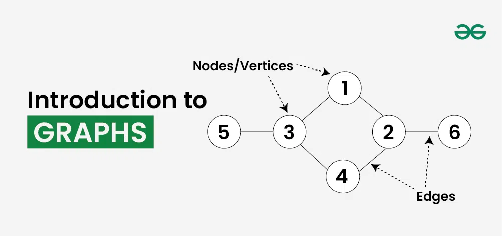
Graph is a non-linear data structure consisting of vertices and edges. The vertices are sometimes also referred to as nodes and the edges are lines or arcs that connect any two nodes in the graph. More formally a Graph is composed of a set of vertices( V ) and a set of edges( E ). The graph is denoted by G(V, E).
Imagine a game of football as a web of connections, where players are the nodes and their interactions on the field are the edges. This web of connections is exactly what a graph data structure represents, and it’s the key to unlocking insights into team performance and player dynamics in sports.
Components of a Graph:
- Vertices: Vertices are the fundamental units of the graph. Sometimes, vertices are also known as vertex or nodes. Every node/vertex can be labeled or unlabelled.
- Edges: Edges are drawn or used to connect two nodes of the graph. It can be ordered pair of nodes in a directed graph. Edges can connect any two nodes in any possible way. There are no rules. Sometimes, edges are also known as arcs. Every edge can be labelled/unlabelled.
Types Of Graph
1. Null Graph
A graph is known as a null graph if there are no edges in the graph.
2. Trivial Graph
Graph having only a single vertex, it is also the smallest graph possible. 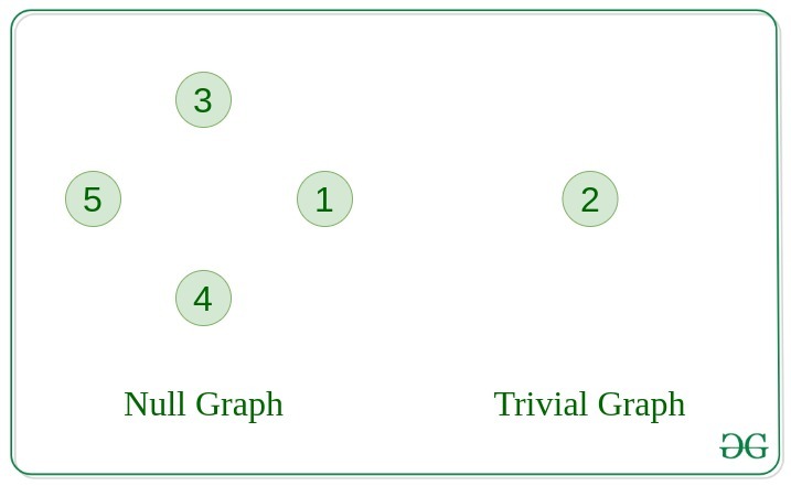
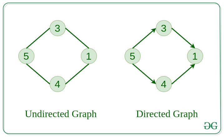
3. Undirected Graph
A graph in which edges do not have any direction. That is the nodes are unordered pairs in the definition of every edge.
4. Directed Graph
A graph in which edge has direction. That is the nodes are ordered pairs in the definition of every edge.
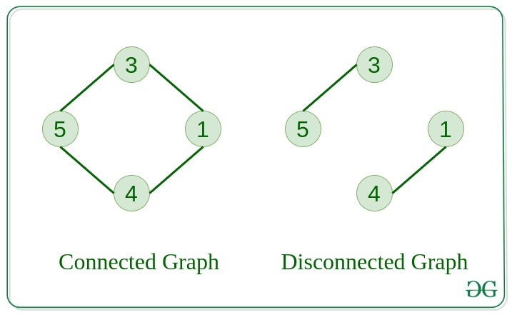
5. Connected Graph
The graph in which from one node we can visit any other node in the graph is known as a connected graph.
6. Disconnected Graph
The graph in which at least one node is not reachable from a node is known as a disconnected graph.
7. Regular Graph
The graph in which the degree of every vertex is equal to K is called K regular graph.
8. Complete Graph
The graph in which from each node there is an edge to each other node. 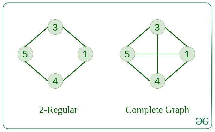
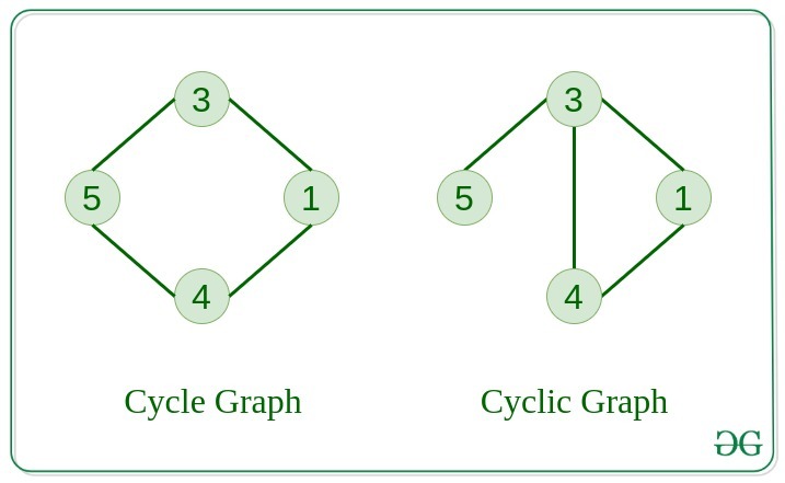
9. Cycle Graph
The graph in which the graph is a cycle in itself, the degree of each vertex is 2.
10. Cyclic Graph
A graph containing at least one cycle is known as a Cyclic graph.
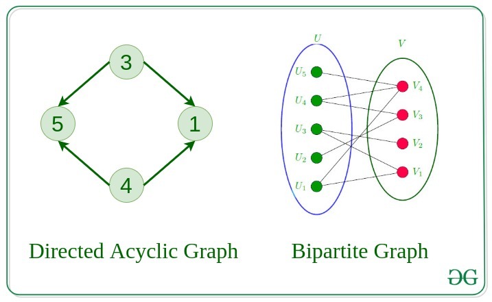
11. Directed Acyclic Graph
A Directed Graph that does not contain any cycle.
12. Bipartite Graph
A graph in which vertex can be divided into two sets such that vertex in each set does not contain any edge between them.
13. Weighted Graph
- A graph in which the edges are already specified with suitable weight is known as a weighted graph.
- Weighted graphs can be further classified as directed weighted graphs and undirected weighted graphs.
Representation of Graphs:
There are two ways to store a graph:
- Adjacency Matrix
- Adjacency List
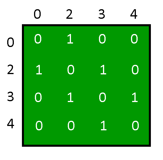
In this method, the graph is stored in the form of the 2D matrix where rows and columns denote vertices. Each entry in the matrix represents the weight of the edge between those vertices.
-copy.webp)
Below is the implementation of Graphs represented using Adjacency Matrix:
#include <iostream>
#include <vector>

using namespace std;

vector<vector<int> >
createAdjacencyMatrix(vector<vector<int> >& graph,
                      int numVertices)
{
    // Initialize the adjacency matrix with zeros
    vector<vector<int> > adjMatrix(
        numVertices, vector<int>(numVertices, 0));

    // Fill the adjacency matrix based on the edges in the
    // graph
    for (int i = 0; i < numVertices; ++i) {
        for (int j = 0; j < numVertices; ++j) {
            if (graph[i][j] == 1) {
                adjMatrix[i][j] = 1;
                adjMatrix[j][i]
                    = 1; // For undirected graph, set
                         // symmetric entries
            }
        }
    }

    return adjMatrix;
}

int main()
{
    // The indices represent the vertices, and the values
    // are lists of neighboring vertices
    vector<vector<int> > graph = { { 0, 1, 0, 0 },
                                   { 1, 0, 1, 0 },
                                   { 0, 1, 0, 1 },
                                   { 0, 0, 1, 0 } };

    int numVertices = graph.size();

    // Create the adjacency matrix
    vector<vector<int> > adjMatrix
        = createAdjacencyMatrix(graph, numVertices);

    // Print the adjacency matrix
    for (int i = 0; i < numVertices; ++i) {
        for (int j = 0; j < numVertices; ++j) {
            cout << adjMatrix[i][j] << " ";
        }
        cout << endl;
    }

    return 0;
}
import java.util.ArrayList;
import java.util.Arrays;

public class AdjacencyMatrix {
    public static int[][] createAdjacencyMatrix(
        ArrayList<ArrayList<Integer> > graph,
        int numVertices)
    {
        // Initialize the adjacency matrix with zeros
        int[][] adjMatrix
            = new int[numVertices][numVertices];

        // Fill the adjacency matrix based on the edges in
        // the graph
        for (int i = 0; i < numVertices; ++i) {
            for (int j = 0; j < numVertices; ++j) {
                if (graph.get(i).get(j) == 1) {
                    adjMatrix[i][j] = 1;
                    adjMatrix[j][i]
                        = 1; // For undirected graph, set
                             // symmetric entries
                }
            }
        }

        return adjMatrix;
    }

    public static void main(String[] args)
    {
        // The indices represent the vertices, and the
        // values are lists of neighboring vertices
        ArrayList<ArrayList<Integer> > graph
            = new ArrayList<>();
        graph.add(
            new ArrayList<>(Arrays.asList(0, 1, 0, 0)));
        graph.add(
            new ArrayList<>(Arrays.asList(1, 0, 1, 0)));
        graph.add(
            new ArrayList<>(Arrays.asList(0, 1, 0, 1)));
        graph.add(
            new ArrayList<>(Arrays.asList(0, 0, 1, 0)));

        int numVertices = graph.size();

        // Create the adjacency matrix
        int[][] adjMatrix
            = createAdjacencyMatrix(graph, numVertices);

        // Print the adjacency matrix
        for (int i = 0; i < numVertices; ++i) {
            for (int j = 0; j < numVertices; ++j) {
                System.out.print(adjMatrix[i][j] + " ");
            }
            System.out.println();
        }
    }
}

// This code is contributed by shivamgupta310570
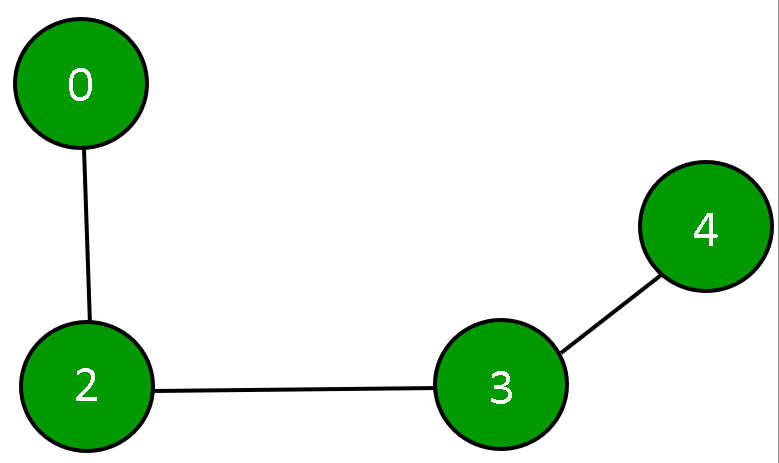
This graph is represented as a collection of linked lists. There is an array of pointer which points to the edges connected to that vertex.
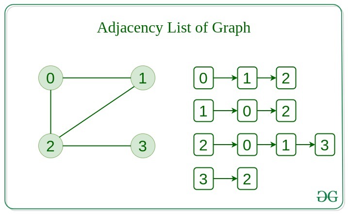
Below is the implementation of Graphs represented using Adjacency List:
#include <bits/stdc++.h>

using namespace std;

vector<vector<int>> createAdjacencyList(vector<vector<int> >& edges, int numVertices)
{
    // Initialize the adjacency list
    vector<vector<int> > adjList(numVertices);

    // Fill the adjacency list based on the edges in the
    // graph
    for (int i=0; i < edges.size(); i++) {
        int u = edges[i][0];
          int v = edges[i][1];
          // Since the graph is undirected, therefore we push the edges in both the directions
          adjList[u].push_back(v);
          adjList[v].push_back(u);
    }

    return adjList;
}

int main()
{
      // Undirected Graph of 4 nodes
      int numVertices = 4;
      vector<vector<int>> edges = {{0, 1}, {0, 2}, {1, 2}, {2, 3}, {3, 1}};

    // Create the adjacency List
    vector<vector<int>> adjList = createAdjacencyList(edges, numVertices);

    // Print the adjacency List
    for (int i = 0; i < numVertices; ++i) {
          cout << i << " -> ";
        for (int j = 0; j < adjList[i].size(); ++j) {
            cout << adjList[i][j] << " ";
        }
        cout << endl;
    }

    return 0;
}
import java.util.ArrayList;
import java.util.List;

public class Main {
    public static List<List<Integer> >
    createAdjacencyList(List<List<Integer> > edges,
                        int numVertices)
    {
        // Initialize the adjacency list
        List<List<Integer> > adjList
            = new ArrayList<>(numVertices);
        for (int i = 0; i < numVertices; i++) {
            adjList.add(new ArrayList<>());
        }

        // Fill the adjacency list based on the edges in the
        // graph
        for (List<Integer> edge : edges) {
            int u = edge.get(0);
            int v = edge.get(1);
            // Since the graph is undirected, therefore we
            // push the edges in both the directions
            adjList.get(u).add(v);
            adjList.get(v).add(u);
        }

        return adjList;
    }

    public static void main(String[] args)
    {
        // Undirected Graph of 4 nodes
        int numVertices = 4;
        List<List<Integer> > edges = new ArrayList<>();
        edges.add(List.of(0, 1));
        edges.add(List.of(0, 2));
        edges.add(List.of(1, 2));
        edges.add(List.of(2, 3));
        edges.add(List.of(3, 1));

        // Create the adjacency list
        List<List<Integer> > adjList
            = createAdjacencyList(edges, numVertices);

        // Print the adjacency list
        for (int i = 0; i < numVertices; ++i) {
            System.out.print(i + " -> ");
            for (int j = 0; j < adjList.get(i).size();
                 ++j) {
                System.out.print(adjList.get(i).get(j)
                                 + " ");
            }
            System.out.println();
        }
    }
}
Output0 -> 1 2
1 -> 0 2 3
2 -> 0 1 3
3 -> 2 1
Comparison between Adjacency Matrix and Adjacency List
When the graph contains a large number of edges then it is good to store it as a matrix because only some entries in the matrix will be empty. An algorithm such as Prim’s and Dijkstra adjacency matrix is used to have less complexity.
| Action | Adjacency Matrix | Adjacency List |
|---|
| Adding Edge | O(1) | O(1) |
| Removing an edge | O(1) | O(N) |
| Initializing | O(N*N) | O(N) |
Basic Operations on Graphs
Below are the basic operations on the graph:
- Insertion or Deletion of Nodes in the graph
- Insertion or Deletion of Edges in the graph
- Searching on Graphs – Search an entity in the graph.
- Traversal of Graphs – Traversing all the nodes in the graph.
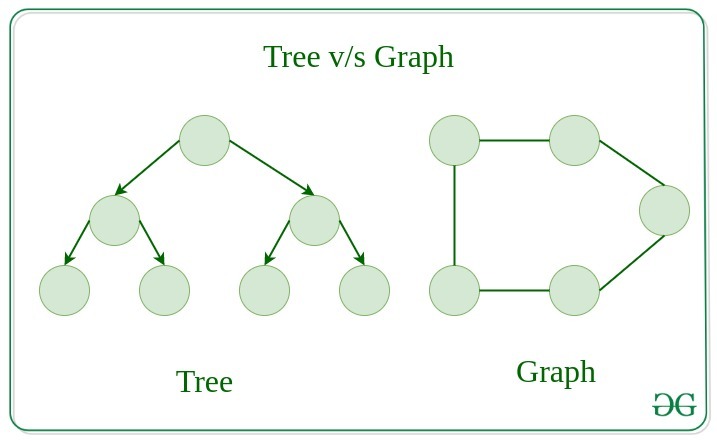
Difference between Tree and Graph:
Trees are the restricted types of graphs, just with some more rules. Every tree will always be a graph but not all graphs will be trees. Linked List, Trees, and Heaps all are special cases of graphs.
Real-Life Applications of Graph:
Graphs have numerous real-life applications across various fields. Some of them are listed below: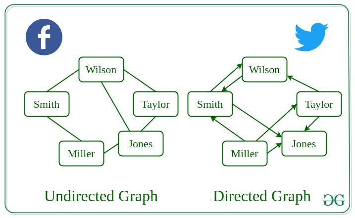
- Graphs are used to represent social networks, such as networks of friends on social media.
- Graphs can be used to represent the topology of computer networks, such as the connections between routers and switches.
- Graphs are used to represent the connections between different places in a transportation network, such as roads and airports.
- Neural Networks: Vertices represent neurons and edges represent the synapses between them. Neural networks are used to understand how our brain works and how connections change when we learn. The human brain has about 10^11 neurons and close to 10^15 synapses.
- Compilers: Graphs are used extensively in compilers. They can be used for type inference, for so-called data flow analysis, register allocation, and many other purposes. They are also used in specialized compilers, such as query optimization in database languages.
- Robot planning: Vertices represent states the robot can be in and the edges the possible transitions between the states. Such graph plans are used, for example, in planning paths for autonomous vehicles.
Advantages of Graphs:
- Graphs are a versatile data structure that can be used to represent a wide range of relationships and data structures.
- They can be used to model and solve a wide range of problems, including pathfinding, data clustering, network analysis, and machine learning.
- Graph algorithms are often very efficient and can be used to solve complex problems quickly and effectively.
- Graphs can be used to represent complex data structures in a simple and intuitive way, making them easier to understand and analyze.
Disadvantages of Graphs:
- Graphs can be complex and difficult to understand, especially for people who are not familiar with graph theory or related algorithms.
- Creating and manipulating graphs can be computationally expensive, especially for very large or complex graphs.
- Graph algorithms can be difficult to design and implement correctly, and can be prone to bugs and errors.
- Graphs can be difficult to visualize and analyze, especially for very large or complex graphs, which can make it challenging to extract meaningful insights from the data.
Frequently Asked Questions(FAQs) on Graphs:
1. What is a graph?
A graph is a data structure consisting of a set of vertices (nodes) and a set of edges that connect pairs of vertices.
2. What are the different types of graphs?
Graphs can be classified into various types based on properties such as directionality of edges (directed or undirected), presence of cycles (acyclic or cyclic), and whether multiple edges between the same pair of vertices are allowed (simple or multigraph).
3. What are the applications of graphs?
Graphs have numerous applications in various fields, including social networks, transportation networks, computer networks, recommendation systems, biology, chemistry, and more.
4. What is the difference between a directed graph and an undirected graph?
In an undirected graph, edges have no direction, meaning they represent symmetric relationships between vertices. In a directed graph (or digraph), edges have a direction, indicating a one-way relationship between vertices.
5. What is a weighted graph?
A weighted graph is a graph in which each edge is assigned a numerical weight or cost. These weights can represent distances, costs, or any other quantitative measure associated with the edges.
6. What is the degree of a vertex in a graph?
The degree of a vertex in a graph is the number of edges incident to that vertex. In a directed graph, the indegree of a vertex is the number of incoming edges, and the outdegree is the number of outgoing edges.
7. What is a path in a graph?
A path in a graph is a sequence of vertices connected by edges. The length of a path is the number of edges it contains.
8. What is a cycle in a graph?
A cycle in a graph is a path that starts and ends at the same vertex, traversing a sequence of distinct vertices and edges in between.
9. What are spanning trees and minimum spanning trees?
A spanning tree of a graph is a subgraph that is a tree and includes all the vertices of the original graph. A minimum spanning tree (MST) is a spanning tree with the minimum possible sum of edge weights.
10. What algorithms are commonly used to traverse or search graphs?
Common graph traversal algorithms include depth-first search (DFS) and breadth-first search (BFS). These algorithms are used to explore or visit all vertices in a graph, typically starting from a specified vertex. Other algorithms, such as Dijkstra’s algorithm and Bellman-Ford algorithm, are used for shortest path finding.
Conclusion:
- Graph data structures are a powerful tool for representing and analyzing relationships between objects or entities.
- Graphs can be used to represent the interactions between different objects or entities, and then analyze these interactions to identify patterns, clusters, communities, key players, influencers, bottlenecks and anomalies.
- In sports data science, graph data structures can be used to analyze and understand the dynamics of team performance and player interactions on the field.
- They can be used in a variety of fields such as Sports, Social media, transportation, cybersecurity and many more.
More Resources of Graph:
------
Add and Remove vertex in Adjacency List representation of Graph
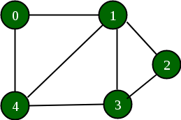
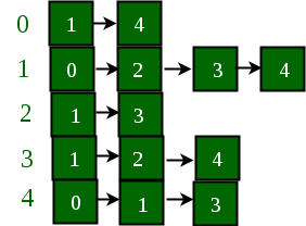
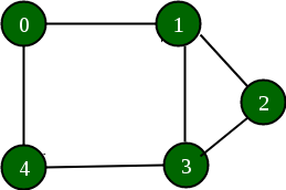
Prerequisites: Linked List, Graph Data Structure In this article, adding and removing a vertex is discussed in a given adjacency list representation. Let the Directed Graph be: 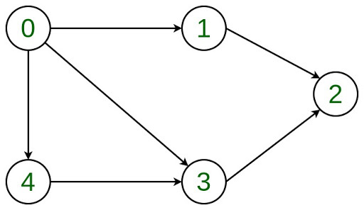 The graph can be represented in the Adjacency List representation as:
 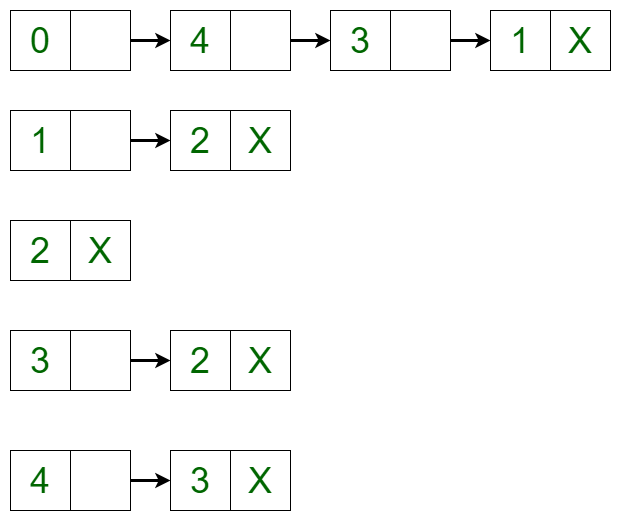 It is a Linked List representation where the head of the linked list is a vertex in the graph and all the connected nodes are the vertices to which the first vertex is connected. For example, from the graph, it is clear that vertex 0 is connected to vertex 4, 3 and 1. The same is representated in the adjacency list(or Linked List) representation.
Approach:
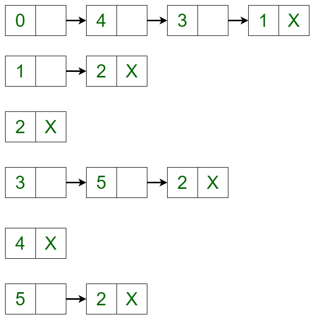
- Adding a Vertex in the Graph: To add a vertex in the graph, the adjacency list can be iterated to the place where the insertion is required and the new node can be created using linked list implementation. For example, if 5 needs to be added between vertex 2 and vertex 3 such that vertex 3 points to vertex 5 and vertex 5 points to vertex 2, then a new edge is created between vertex 5 and vertex 3 and a new edge is created from vertex 5 and vertex 2. After adding the vertex, the adjacency list changes to:
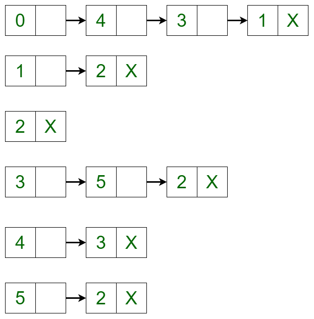
- Removing a Vertex in the Graph: To delete a vertex in the graph, iterate through the list of each vertex if an edge is present or not. If the edge is present, then delete the vertex in the same way as delete is performed in a linked list. For example, the adjacency list translates to the below list if vertex 4 is deleted from the list:
 Below is the implementation of the above approach:
C++
#include <iostream>
using namespace std;
class AdjNode {
public:
int vertex;
AdjNode* next;
AdjNode(int data) {
vertex = data;
next = NULL;
}
};
class AdjList {
private:
int v;
AdjNode** graph;
public:
AdjList(int vertices) {
v = vertices;
graph = new AdjNode*[v];
for (int i = 0; i < v; ++i)
graph[i] = NULL;
}
void addEdge(int source, int destination) {
AdjNode* node = new AdjNode(destination);
node->next = graph;
graph = node;
}
void addVertex(int vk, int source, int destination) {
addEdge(source, vk);
addEdge(vk, destination);
}
void printGraph() {
for (int i = 0; i < v; ++i) {
cout << i << " ";
AdjNode* temp = graph[i];
while (temp != NULL) {
cout << "-> " << temp->vertex << " ";
temp = temp->next;
}
cout << endl;
}
}
void delVertex(int k) {
for (int i = 0; i < v; ++i) {
AdjNode* temp = graph[i];
if (i == k) {
graph[i] = temp->next;
temp = graph[i];
}
while (temp != NULL) {
if (temp->vertex == k) {
break;
}
AdjNode* prev = temp;
temp = temp->next;
if (temp == NULL) {
continue;
}
prev->next = temp->next;
temp = NULL;
}
}
}
};
int main() {
int V = 6;
AdjList graph(V);
graph.addEdge(0, 1);
graph.addEdge(0, 3);
graph.addEdge(0, 4);
graph.addEdge(1, 2);
graph.addEdge(3, 2);
graph.addEdge(4, 3);
cout << "Initial adjacency list" << endl;
graph.printGraph();
graph.addVertex(5, 3, 2);
cout << "Adjacency list after adding vertex" << endl;
graph.printGraph();
graph.delVertex(4);
cout << "Adjacency list after deleting vertex" << endl;
graph.printGraph();
return 0;
}
|
Java
import java.util.*;
class AdjNode {
int vertex;
AdjNode next;
public AdjNode(int data)
{
vertex = data;
next = null;
}
}
class AdjList {
private int v;
private AdjNode[] graph;
public AdjList(int vertices)
{
v = vertices;
graph = new AdjNode[v];
for (int i = 0; i < v; ++i) {
graph[i] = null;
}
}
public void addEdge(int source, int destination)
{
AdjNode node = new AdjNode(destination);
node.next = graph;
graph = node;
}
public void addVertex(int vk, int source,
int destination)
{
addEdge(source, vk);
addEdge(vk, destination);
}
public void printGraph()
{
for (int i = 0; i < v; ++i) {
System.out.print(i + " ");
AdjNode temp = graph[i];
while (temp != null) {
System.out.print("-> " + temp.vertex + " ");
temp = temp.next;
}
System.out.println();
}
}
public void delVertex(int k)
{
for (int i = 0; i < v; ++i) {
AdjNode temp = graph[i];
if (i == k) {
graph[i] = temp.next;
temp = graph[i];
}
while (temp != null) {
if (temp.vertex == k) {
break;
}
AdjNode prev = temp;
temp = temp.next;
if (temp == null) {
continue;
}
prev.next = temp.next;
temp = null;
}
}
}
}
public class Main {
public static void main(String[] args)
{
int V = 6;
AdjList graph = new AdjList(V);
graph.addEdge(0, 1);
graph.addEdge(0, 3);
graph.addEdge(0, 4);
graph.addEdge(1, 2);
graph.addEdge(3, 2);
graph.addEdge(4, 3);
System.out.println("Initial adjacency list");
graph.printGraph();
graph.addVertex(5, 3, 2);
System.out.println(
"Adjacency list after adding vertex");
graph.printGraph();
graph.delVertex(4);
System.out.println(
"Adjacency list after deleting vertex");
graph.printGraph();
}
}
|
Python3
class AdjNode(object):
def __init__(self, data):
self.vertex = data
self.next = None
class AdjList(object):
def __init__(self, vertices):
self.v = vertices
self.graph = [None] * self.v
def addedge(self, source, destination):
node = AdjNode(destination)
node.next = self.graph
self.graph = node
def addvertex(self, vk, source, destination):
self.addedge(source, vk)
self.addedge(vk, destination)
def print_graph(self):
for i in range(self.v):
print(i, end=" ")
temp = self.graph[i]
while temp:
print("->", temp.vertex, end=" ")
temp = temp.next
print("\n")
def delvertex(self, k):
for i in range(self.v):
temp = self.graph[i]
if i == k:
self.graph[i] = temp.next
temp = self.graph[i]
if temp:
if temp.vertex == k:
self.graph[i] = temp.next
temp = None
while temp:
if temp.vertex == k:
break
prev = temp
temp = temp.next
if temp == None:
continue
prev.next = temp.next
temp = None
if __name__ == "__main__":
V = 6
graph = AdjList(V)
graph.addedge(0, 1)
graph.addedge(0, 3)
graph.addedge(0, 4)
graph.addedge(1, 2)
graph.addedge(3, 2)
graph.addedge(4, 3)
print("Initial adjacency list")
graph.print_graph()
graph.addvertex(5, 3, 2)
print("Adjacency list after adding vertex")
graph.print_graph()
graph.delvertex(4)
print("Adjacency list after deleting vertex")
graph.print_graph()
|
C#
using System;
class AdjNode {
public int vertex;
public AdjNode next;
public AdjNode(int data)
{
vertex = data;
next = null;
}
}
class AdjList {
private int v;
private AdjNode[] graph;
public AdjList(int vertices)
{
v = vertices;
graph = new AdjNode[v];
for (int i = 0; i < v; ++i) {
graph[i] = null;
}
}
public void addEdge(int source, int destination)
{
AdjNode node = new AdjNode(destination);
node.next = graph;
graph = node;
}
public void addVertex(int vk, int source,
int destination)
{
addEdge(source, vk);
addEdge(vk, destination);
}
public void printGraph()
{
for (int i = 0; i < v; ++i) {
Console.Write(i + " ");
AdjNode temp = graph[i];
while (temp != null) {
Console.Write("-> " + temp.vertex + " ");
temp = temp.next;
}
Console.WriteLine();
}
}
public void delVertex(int k)
{
for (int i = 0; i < v; ++i) {
AdjNode temp = graph[i];
if (i == k) {
graph[i] = temp.next;
temp = graph[i];
}
while (temp != null) {
if (temp.vertex == k) {
break;
}
AdjNode prev = temp;
temp = temp.next;
if (temp == null) {
continue;
}
prev.next = temp.next;
temp = null;
}
}
}
}
public class GFG {
static public void Main()
{
int V = 6;
AdjList graph = new AdjList(V);
graph.addEdge(0, 1);
graph.addEdge(0, 3);
graph.addEdge(0, 4);
graph.addEdge(1, 2);
graph.addEdge(3, 2);
graph.addEdge(4, 3);
Console.WriteLine("Initial adjacency list");
graph.printGraph();
graph.addVertex(5, 3, 2);
Console.WriteLine(
"Adjacency list after adding vertex");
graph.printGraph();
graph.delVertex(4);
Console.WriteLine(
"Adjacency list after deleting vertex");
graph.printGraph();
}
}
|
Javascript
<script>
class AdjNode {
constructor(data) {
this.vertex = data;
this.next = null;
}
}
class AdjList {
constructor(vertices) {
this.v = vertices;
this.graph = new Array(this.v).fill(null);
}
addEdge(source, destination) {
const node = new AdjNode(destination);
node.next = this.graph;
this.graph = node;
}
addVertex(vk, source, destination) {
this.addEdge(source, vk);
this.addEdge(vk, destination);
}
printGraph() {
for (let i = 0; i < this.v; ++i) {
let str = i + " ";
let temp = this.graph[i];
while (temp != null) {
str += "-> " + temp.vertex + " ";
temp = temp.next;
}
document.write(str + "<br>");
}
}
delVertex(k) {
for (let i = 0; i < this.v; ++i) {
let temp = this.graph[i];
if (i === k) {
this.graph[i] = temp.next;
temp = this.graph[i];
}
while (temp != null) {
if (temp.vertex === k) {
break;
}
let prev = temp;
temp = temp.next;
if (temp == null) {
continue;
}
prev.next = temp.next;
temp = null;
}
}
}
}
const V = 6;
const graph = new AdjList(V);
graph.addEdge(0, 1);
graph.addEdge(0, 3);
graph.addEdge(0, 4);
graph.addEdge(1, 2);
graph.addEdge(3, 2);
graph.addEdge(4, 3);
document.write("Initial adjacency list<br>");
graph.printGraph();
graph.addVertex(5, 3, 2);
document.write("Adjacency list after adding vertex<br>");
graph.printGraph();
graph.delVertex(4);
document.write("Adjacency list after deleting vertex<br>");
graph.printGraph();
</script>
|
Output
Initial adjacency list
0-> 4-> 3-> 1

1-> 2

2

3-> 2

4-> 3

5

Adjacency list after adding vertex
0-> 4-> 3-> 1

1-> 2

2

3-> 5-> 2

4-> 3

5-> 2

Adjacency list after deleting vertex
0-> 3-> 1

1-> 2

2

3-> 5-> 2

4

5-> 2
------
Add and Remove vertex in Adjacency Matrix representation of Graph
A graph is a presentation of a set of entities where some pairs of entities are linked by a connection. Interconnected entities are represented by points referred to as vertices, and the connections between the vertices are termed as edges. Formally, a graph is a pair of sets (V, E), where V is a collection of vertices, and E is a collection of edges joining a pair of vertices.
A graph can be represented by using an Adjacency Matrix.
Initialization of Graph: The adjacency matrix will be depicted using a 2D array, a constructor will be used to assign the size of the array and each element of that array will be initialized to 0. Showing that the degree of each vertex in the graph is zero.
C++
class Graph {
private:
int n;
int g[10][10];
public:
Graph(int x)
{
n = x;
for (int i = 0; i < n; ++i) {
for (int j = 0; j < n; ++j) {
g[i][j] = 0;
}
}
}
};
|
Java
class Graph {
private int n;
private int[][] g = new int[10][10];
Graph(int x)
{
this.n = x;
int i, j;
for (i = 0; i < n; ++i) {
for (j = 0; j < n; ++j) {
g[i][j] = 0;
}
}
}
}
|
Python3
class Graph:
__n = 0
__g =[[0 for x in range(10)] for y in range(10)]
def __init__(self, x):
self.__n = x
for i in range(0, self.__n):
for j in range(0, self.__n):
self.__g[i][j]= 0
|
C#
class Graph{
private int n;
private int[,] g = new int[10, 10];
Graph(int x)
{
this.n = x;
int i, j;
for(i = 0; i < n; ++i)
{
for(j = 0; j < n; ++j)
{
g[i, j] = 0;
}
}
}
}
|
Javascript
class Graph {
constructor(x) {
this.n = x;
this.g = [];
for (let i = 0; i < this.n; ++i) {
this.g[i] = [];
for (let j = 0; j < this.n; ++j) {
this.g[i][j] = 0;
}
}
}
}
|
Here the adjacency matrix is g[n][n] in which the degree of each vertex is zero.
Displaying the Graph: The graph is depicted using the adjacency matrix g[n][n] having the number of vertices n. The 2D array(adjacency matrix) is displayed in which if there is an edge between two vertices ‘x’ and ‘y’ then g[x][y] is 1 otherwise 0.
C++
void displayAdjacencyMatrix()
{
cout << "\n\n Adjacency Matrix:";
for (int i = 0; i < n; ++i) {
cout << "\n";
for (int j = 0; j < n; ++j) {
cout << " " << g[i][j];
}
}
}
|
Java
public void displayAdjacencyMatrix()
{
System.out.print("\n\n Adjacency Matrix:");
for (int i = 0; i < n; ++i) {
System.out.println();
for (int j = 0; j < n; ++j) {
System.out.print(" " + g[i][j]);
}
}
}
|
Python3
def displayAdjacencyMatrix(self):
print("\n\n Adjacency Matrix:", end ="")
for i in range(0, self.__n):
print()
for j in range(0, self.__n):
print("", self.__g[i][j], end ="")
|
C#
public void DisplayAdjacencyMatrix()
{
Console.Write("\n\n Adjacency Matrix:");
for (int i = 0; i < n; ++i)
{
Console.WriteLine();
for (int j = 0; j < n; ++j)
{
Console.Write(" " + g[i,j]);
}
}
}
|
Javascript
function displayAdjacencyMatrix() {
console.log("\n\n Adjacency Matrix:");
for (let i = 0; i < n; ++i) {
let row = "";
for (let j = 0; j < n; ++j) {
row += " " + g[i][j];
}
console.log(row);
}
}
|
The above method is a public member function of the class Graph which displays the graph using an adjacency matrix.
Adding Edges between Vertices in the Graph: To add edges between two existing vertices such as vertex ‘x’ and vertex ‘y’ then the elements g[x][y] and g[y][x] of the adjacency matrix will be assigned to 1, depicting that there is an edge between vertex ‘x’ and vertex ‘y’.
C++
void addEdge(int x, int y)
{
if ((x >= n) || (y > n)) {
cout << "Vertex does not exists!";
}
if (x == y) {
cout << "Same Vertex!";
}
else {
g[y][x] = 1;
g[x][y] = 1;
}
}
|
Java
public void addEdge(int x, int y)
{
if ((x >= n) || (y > n)) {
System.out.println("Vertex does not exists!");
}
if (x == y) {
System.out.println("Same Vertex!");
}
else {
g[y][x] = 1;
g[x][y] = 1;
}
}
|
Python3
def addEdge(self, x, y):
if(x>= self.__n) or (y >= self.__n):
print("Vertex does not exists !")
if(x == y):
print("Same Vertex !")
else:
self.__g[y][x]= 1
self.__g[x][y]= 1
|
C#
public void AddEdge(int x, int y)
{
if ((x >= n) || (y > n))
{
Console.WriteLine("Vertex does not exists!");
}
if (x == y)
{
Console.WriteLine("Same Vertex!");
}
else
{
g[y, x] = 1;
g[x, y] = 1;
}
}
|
Javascript
function addEdge(x, y) {
if ((x >= n) || (y > n)) {
console.log("Vertex does not exist!");
}
if (x === y) {
console.log("Same Vertex!");
}
else {
g[y][x] = 1;
g[x][y] = 1;
}
}
|
Here the above method is a public member function of the class Graph which connects any two existing vertices in the Graph.
Adding a Vertex in the Graph: To add a vertex in the graph, we need to increase both the row and column of the existing adjacency matrix and then initialize the new elements related to that vertex to 0.(i.e the new vertex added is not connected to any other vertex)
C++
void addVertex()
{
n++;
int i;
for (i = 0; i < n; ++i) {
g[i][n - 1] = 0;
g[n - 1][i] = 0;
}
}
|
Java
public void addVertex()
{
n++;
int i;
for (i = 0; i < n; ++i) {
g[i][n - 1] = 0;
g[n - 1][i] = 0;
}
}
|
Python3
def addVertex(self):
self.__n = self.__n + 1;
for i in range(0, self.__n):
self.__g[i][self.__n-1]= 0
self.__g[self.__n-1][i]= 0
|
Javascript
function addVertex() {
n++;
let i;
for (i = 0; i < n; ++i) {
g[i][n - 1] = 0;
g[n - 1][i] = 0;
}
}
|
C#
public void addVertex()
{
n++;
int i;
for (i = 0; i < n; ++i) {
g[i, n - 1] = 0;
g[n - 1, i] = 0;
}
}
|
The above method is a public member function of the class Graph which increments the number of vertices by 1 and the degree of the new vertex is 0.
Removing a Vertex in the Graph: To remove a vertex from the graph, we need to check if that vertex exists in the graph or not and if that vertex exists then we need to shift the rows to the left and the columns upwards of the adjacency matrix so that the row and column values of the given vertex gets replaced by the values of the next vertex and then decrease the number of vertices by 1.In this way that particular vertex will be removed from the adjacency matrix.
C++
void removeVertex(int x)
{
if (x > n) {
cout << "\nVertex not present!";
return;
}
else {
int i;
while (x < n) {
for (i = 0; i < n; ++i) {
g[i][x] = g[i][x + 1];
}
for (i = 0; i < n; ++i) {
g[x][i] = g[x + 1][i];
}
x++;
}
n--;
}
}
|
Java
public void removeVertex(int x)
{
if (x > n) {
System.out.println("Vertex not present!");
return;
}
else {
int i;
while (x < n) {
for (i = 0; i < n; ++i) {
g[i][x] = g[i][x + 1];
}
for (i = 0; i < n; ++i) {
g[x][i] = g[x + 1][i];
}
x++;
}
n--;
}
}
|
Python3
def removeVertex(self, x):
if(x>self.__n):
print("Vertex not present !")
else:
while(x<self.__n):
for i in range(0, self.__n):
self.__g[i][x]= self.__g[i][x + 1]
for i in range(0, self.__n):
self.__g[x][i]= self.__g[x + 1][i]
x = x + 1
self.__n = self.__n - 1
|
C#
public void RemoveVertex(int x)
{
if (x > n) {
Console.WriteLine("Vertex not present!");
return;
}
else {
int i;
while (x < n) {
for (i = 0; i < n; ++i) {
g[i][x] = g[i][x + 1];
}
for (i = 0; i < n; ++i) {
g[x][i] = g[x + 1][i];
}
x++;
}
n--;
}
}
|
Javascript
function removeVertex(x) {
if (x > n) {
console.log("\nVertex not present!");
return;
} else {
let i;
while (x < n) {
for (i = 0; i < n; ++i) {
g[i][x] = g[i][x + 1];
}
for (i = 0; i < n; ++i) {
g[x][i] = g[x + 1][i];
}
x++;
}
n--;
}
}
|
The above method is a public member function of the class Graph which removes an existing vertex from the graph by shifting the rows to the left and shifting the columns up to replace the row and column values of that vertex with the next vertex and then decreases the number of vertices by 1 in the graph.
Following is a complete program that uses all of the above methods in a Graph.
C++
#include <iostream>
using namespace std;
class Graph {
private:
int n;
int g[10][10];
public:
Graph(int x)
{
n = x;
for (int i = 0; i < n; ++i) {
for (int j = 0; j < n; ++j) {
g[i][j] = 0;
}
}
}
void displayAdjacencyMatrix()
{
cout << "\n\n Adjacency Matrix:";
for (int i = 0; i < n; ++i) {
cout << "\n";
for (int j = 0; j < n; ++j) {
cout << " " << g[i][j];
}
}
}
void addEdge(int x, int y)
{
if ((x >= n) || (y > n)) {
cout << "Vertex does not exists!";
}
if (x == y) {
cout << "Same Vertex!";
}
else {
g[y][x] = 1;
g[x][y] = 1;
}
}
void addVertex()
{
n++;
int i;
for (i = 0; i < n; ++i) {
g[i][n - 1] = 0;
g[n - 1][i] = 0;
}
}
void removeVertex(int x)
{
if (x > n) {
cout << "\nVertex not present!";
return;
}
else {
int i;
while (x < n) {
for (i = 0; i < n; ++i) {
g[i][x] = g[i][x + 1];
}
for (i = 0; i < n; ++i) {
g[x][i] = g[x + 1][i];
}
x++;
}
n--;
}
}
};
int main()
{
Graph obj(4);
obj.addEdge(0, 1);
obj.addEdge(0, 2);
obj.addEdge(1, 2);
obj.addEdge(2, 3);
obj.displayAdjacencyMatrix();
obj.addVertex();
obj.addEdge(4, 1);
obj.addEdge(4, 3);
obj.displayAdjacencyMatrix();
obj.removeVertex(1);
obj.displayAdjacencyMatrix();
return 0;
}
|
Java
class Graph
{
private int n;
private int[][] g = new int[10][10];
Graph(int x)
{
this.n = x;
int i, j;
for (i = 0; i < n; ++i)
{
for (j = 0; j < n; ++j)
{
g[i][j] = 0;
}
}
}
public void displayAdjacencyMatrix()
{
System.out.print("\n\n Adjacency Matrix:");
for (int i = 0; i < n; ++i)
{
System.out.println();
for (int j = 0; j < n; ++j)
{
System.out.print(" " + g[i][j]);
}
}
}
public void addEdge(int x, int y)
{
if ((x >= n) || (y > n))
{
System.out.println("Vertex does not exists!");
}
if (x == y)
{
System.out.println("Same Vertex!");
}
else
{
g[y][x] = 1;
g[x][y] = 1;
}
}
public void addVertex()
{
n++;
int i;
for (i = 0; i < n; ++i)
{
g[i][n - 1] = 0;
g[n - 1][i] = 0;
}
}
public void removeVertex(int x)
{
if (x > n)
{
System.out.println("Vertex not present!");
return;
}
else
{
int i;
while (x < n)
{
for (i = 0; i < n; ++i)
{
g[i][x] = g[i][x + 1];
}
for (i = 0; i < n; ++i)
{
g[x][i] = g[x + 1][i];
}
x++;
}
n--;
}
}
}
class Main
{
public static void main(String[] args)
{
Graph obj = new Graph(4);
obj.addEdge(0, 1);
obj.addEdge(0, 2);
obj.addEdge(1, 2);
obj.addEdge(2, 3);
obj.displayAdjacencyMatrix();
obj.addVertex();
obj.addEdge(4, 1);
obj.addEdge(4, 3);
obj.displayAdjacencyMatrix();
obj.removeVertex(1);
obj.displayAdjacencyMatrix();
}
}
|
Python3
class Graph:
__n = 0
__g =[[0 for x in range(10)] for y in range(10)]
def __init__(self, x):
self.__n = x
for i in range(0, self.__n):
for j in range(0, self.__n):
self.__g[i][j]= 0
def displayAdjacencyMatrix(self):
print("\n\n Adjacency Matrix:", end ="")
for i in range(0, self.__n):
print()
for j in range(0, self.__n):
print("", self.__g[i][j], end ="")
def addEdge(self, x, y):
if(x>= self.__n) or (y >= self.__n):
print("Vertex does not exists !")
if(x == y):
print("Same Vertex !")
else:
self.__g[y][x]= 1
self.__g[x][y]= 1
def addVertex(self):
self.__n = self.__n + 1;
for i in range(0, self.__n):
self.__g[i][self.__n-1]= 0
self.__g[self.__n-1][i]= 0
def removeVertex(self, x):
if(x>self.__n):
print("Vertex not present !")
else:
while(x<self.__n):
for i in range(0, self.__n):
self.__g[i][x]= self.__g[i][x + 1]
for i in range(0, self.__n):
self.__g[x][i]= self.__g[x + 1][i]
x = x + 1
self.__n = self.__n - 1
obj = Graph(4);
obj.addEdge(0, 1);
obj.addEdge(0, 2);
obj.addEdge(1, 2);
obj.addEdge(2, 3);
obj.displayAdjacencyMatrix();
obj.addVertex();
obj.addEdge(4, 1);
obj.addEdge(4, 3);
obj.displayAdjacencyMatrix();
obj.removeVertex(1);
obj.displayAdjacencyMatrix();
|
C#
using System;
public class Graph
{
private int n;
private int[,] g = new int[10, 10];
public Graph(int x)
{
this.n = x;
int i, j;
for (i = 0; i < n; ++i)
{
for (j = 0; j < n; ++j)
{
g[i, j] = 0;
}
}
}
public void displayAdjacencyMatrix()
{
Console.Write("\n\n Adjacency Matrix:");
for (int i = 0; i < n; ++i)
{
Console.WriteLine();
for (int j = 0; j < n; ++j)
{
Console.Write(" " + g[i, j]);
}
}
}
public void addEdge(int x, int y)
{
if ((x >= n) || (y > n))
{
Console.WriteLine("Vertex does not exists!");
}
if (x == y)
{
Console.WriteLine("Same Vertex!");
}
else
{
g[y, x] = 1;
g[x, y] = 1;
}
}
public void addVertex()
{
n++;
int i;
for (i = 0; i < n; ++i)
{
g[i, n - 1] = 0;
g[n - 1, i] = 0;
}
}
public void removeVertex(int x)
{
if (x > n)
{
Console.WriteLine("Vertex not present!");
return;
}
else
{
int i;
while (x < n)
{
for (i = 0; i < n; ++i)
{
g[i, x] = g[i, x + 1];
}
for (i = 0; i < n; ++i)
{
g[x, i] = g[x + 1, i];
}
x++;
}
n--;
}
}
}
public class GFG
{
public static void Main(String[] args)
{
Graph obj = new Graph(4);
obj.addEdge(0, 1);
obj.addEdge(0, 2);
obj.addEdge(1, 2);
obj.addEdge(2, 3);
obj.displayAdjacencyMatrix();
obj.addVertex();
obj.addEdge(4, 1);
obj.addEdge(4, 3);
obj.displayAdjacencyMatrix();
obj.removeVertex(1);
obj.displayAdjacencyMatrix();
}
}
|
Javascript
<script>
class Graph
{
constructor(x)
{
this.n=x;
this.g = new Array(10);
for(let i=0;i<10;i++)
{
this.g[i]=new Array(10);
for(let j=0;j<10;j++)
{
this.g[i][j]=0;
}
}
}
displayAdjacencyMatrix()
{
document.write("<br><br> Adjacency Matrix:");
for (let i = 0; i < this.n; ++i)
{
document.write("<br>");
for (let j = 0; j < this.n; ++j)
{
document.write(" " + this.g[i][j]);
}
}
}
addEdge(x,y)
{
if ((x >= this.n) || (y > this.n))
{
document.write("Vertex does not exists!<br>");
}
if (x == y)
{
document.write("Same Vertex!<br>");
}
else
{
this.g[y][x] = 1;
this.g[x][y] = 1;
}
}
addVertex()
{
this.n++;
let i;
for (i = 0; i < this.n; ++i)
{
this.g[i][this.n - 1] = 0;
this.g[this.n - 1][i] = 0;
}
}
removeVertex(x)
{
if (x > this.n)
{
document.write("Vertex not present!<br>");
return;
}
else
{
let i;
while (x < this.n)
{
for (i = 0; i < this.n; ++i)
{
this.g[i][x] = this.g[i][x + 1];
}
for (i = 0; i < this.n; ++i)
{
this.g[x][i] = this.g[x + 1][i];
}
x++;
}
this.n--;
}
}
}
let obj = new Graph(4);
obj.addEdge(0, 1);
obj.addEdge(0, 2);
obj.addEdge(1, 2);
obj.addEdge(2, 3);
obj.displayAdjacencyMatrix();
obj.addVertex();
obj.addEdge(4, 1);
obj.addEdge(4, 3);
obj.displayAdjacencyMatrix();
obj.removeVertex(1);
obj.displayAdjacencyMatrix();
</script>
|
Output:
Adjacency Matrix:
0 1 1 0
1 0 1 0
1 1 0 1
0 0 1 0

Adjacency Matrix:
0 1 1 0 0
1 0 1 0 1
1 1 0 1 0
0 0 1 0 1
0 1 0 1 0

Adjacency Matrix:
0 1 0 0
1 0 1 0
0 1 0 1
0 0 1 0
Adjacency matrices waste a lot of memory space. Such matrices are found to be very sparse. This representation requires space for n*n elements, the time complexity of the addVertex() method is O(n), and the time complexity of the removeVertex() method is O(n*n) for a graph of n vertices.
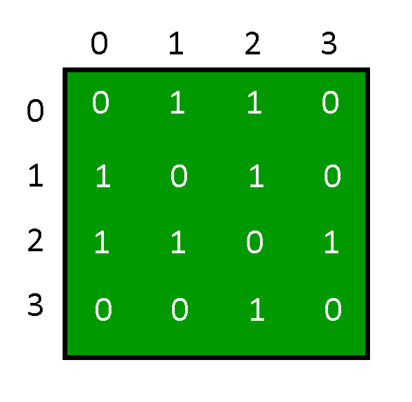
From the output of the program, the Adjacency Matrix is:
And the Graph depicted by the above Adjacency Matrix is:
------
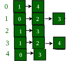
Add and Remove Edge in Adjacency List representation of a Graph
Prerequisites: Graph and Its Representation
In this article, adding and removing edge is discussed in a given adjacency list representation.
A vector has been used to implement the graph using adjacency list representation. It is used to store the adjacency lists of all the vertices. The vertex number is used as the index in this vector.
Example:
Below is a graph and its adjacency list representation:
If the edge between 1 and 4 has to be removed, then the above graph and the adjacency list transforms to:
Approach: The idea is to represent the graph as an array of vectors such that every vector represents adjacency list of the vertex.
- Adding an edge: Adding an edge is done by inserting both of the vertices connected by that edge in each others list. For example, if an edge between (u, v) has to be added, then u is stored in v’s vector list and v is stored in u’s vector list. (push_back)
- Deleting an edge: To delete edge between (u, v), u’s adjacency list is traversed until v is found and it is removed from it. The same operation is performed for v.(erase)
Below is the implementation of the approach:
C++
#include <bits/stdc++.h>
using namespace std;
void addEdge(vector<int> adj[], int u, int v)
{
adj[u].push_back(v);
adj[v].push_back(u);
}
void delEdge(vector<int> adj[], int u, int v)
{
for (int i = 0; i < adj[u].size(); i++) {
if (adj[u][i] == v) {
adj[u].erase(adj[u].begin() + i);
break;
}
}
for (int i = 0; i < adj[v].size(); i++) {
if (adj[v][i] == u) {
adj[v].erase(adj[v].begin() + i);
break;
}
}
}
void printGraph(vector<int> adj[], int V)
{
for (int v = 0; v < V; ++v) {
cout << "vertex " << v << " ";
for (auto x : adj[v])
cout << "-> " << x;
printf("\n");
}
printf("\n");
}
int main()
{
int V = 5;
vector<int> adj[V];
addEdge(adj, 0, 1);
addEdge(adj, 0, 4);
addEdge(adj, 1, 2);
addEdge(adj, 1, 3);
addEdge(adj, 1, 4);
addEdge(adj, 2, 3);
addEdge(adj, 3, 4);
printGraph(adj, V);
delEdge(adj, 1, 4);
printGraph(adj, V);
return 0;
}
|
Java
import java.util.*;
class GFG
{
static void addEdge(Vector<Integer> adj[],
int u, int v)
{
adj[u].add(v);
adj[v].add(u);
}
static void delEdge(Vector<Integer> adj[],
int u, int v)
{
for (int i = 0; i < adj[u].size(); i++)
{
if (adj[u].get(i) == v)
{
adj[u].remove(i);
break;
}
}
for (int i = 0; i < adj[v].size(); i++)
{
if (adj[v].get(i) == u)
{
adj[v].remove(i);
break;
}
}
}
static void printGraph(Vector<Integer> adj[], int V)
{
for (int v = 0; v < V; ++v)
{
System.out.print("vertex " + v+ " ");
for (Integer x : adj[v])
System.out.print("-> " + x);
System.out.printf("\n");
}
System.out.printf("\n");
}
public static void main(String[] args)
{
int V = 5;
Vector<Integer> []adj = new Vector[V];
for (int i = 0; i < V; i++)
adj[i] = new Vector<Integer>();
addEdge(adj, 0, 1);
addEdge(adj, 0, 4);
addEdge(adj, 1, 2);
addEdge(adj, 1, 3);
addEdge(adj, 1, 4);
addEdge(adj, 2, 3);
addEdge(adj, 3, 4);
printGraph(adj, V);
delEdge(adj, 1, 4);
printGraph(adj, V);
}
}
|
Python3
def addEdge(adj, u, v):
adj[u].append(v);
adj[v].append(u);
def delEdge(adj, u, v):
for i in range(len(adj[u])):
if (adj[u][i] == v):
adj[u].pop(i);
break;
for i in range(len(adj[v])):
if (adj[v][i] == u):
adj[v].pop(i);
break;
def prGraph(adj, V):
for v in range(V):
print("vertex " + str(v), end = ' ')
for x in adj[v]:
print("-> " + str(x), end = '')
print()
print()
if __name__=='__main__':
V = 5;
adj = [[] for i in range(V)]
addEdge(adj, 0, 1);
addEdge(adj, 0, 4);
addEdge(adj, 1, 2);
addEdge(adj, 1, 3);
addEdge(adj, 1, 4);
addEdge(adj, 2, 3);
addEdge(adj, 3, 4);
prGraph(adj, V);
delEdge(adj, 1, 4);
prGraph(adj, V);
|
C#
using System;
using System.Collections.Generic;
class GFG
{
static void addEdge(List<int> []adj,
int u, int v)
{
adj[u].Add(v);
adj[v].Add(u);
}
static void delEdge(List<int> []adj,
int u, int v)
{
for (int i = 0; i < adj[u].Count; i++)
{
if (adj[u][i] == v)
{
adj[u].RemoveAt(i);
break;
}
}
for (int i = 0; i < adj[v].Count; i++)
{
if (adj[v][i] == u)
{
adj[v].RemoveAt(i);
break;
}
}
}
static void printGraph(List<int> []adj, int V)
{
for (int v = 0; v < V; ++v)
{
Console.Write("vertex " + v + " ");
foreach (int x in adj[v])
Console.Write("-> " + x);
Console.Write("\n");
}
Console.Write("\n");
}
public static void Main(String[] args)
{
int V = 5;
List<int> []adj = new List<int>[V];
for (int i = 0; i < V; i++)
adj[i] = new List<int>();
addEdge(adj, 0, 1);
addEdge(adj, 0, 4);
addEdge(adj, 1, 2);
addEdge(adj, 1, 3);
addEdge(adj, 1, 4);
addEdge(adj, 2, 3);
addEdge(adj, 3, 4);
printGraph(adj, V);
delEdge(adj, 1, 4);
printGraph(adj, V);
}
}
|
Javascript
const addEdge = (adj, u, v) => {
adj[u].push(v);
adj[v].push(u);
};
const delEdge = (adj, u, v) => {
const indexOfVInU = adj[u].indexOf(v);
adj[u].splice(indexOfVInU, 1);
const indexOfUInV = adj[v].indexOf(u);
adj[v].splice(indexOfUInV, 1);
};
const printGraph = (adj, V) => {
for (let v = 0; v < V; v++) {
console.log(`vertex ${v} `, adj[v].join("-> "));
}
};
const main = () => {
const V = 5;
const adj = [];
for (let i = 0; i < V; i++) {
adj[i] = [];
}
addEdge(adj, 0, 1);
addEdge(adj, 0, 4);
addEdge(adj, 1, 2);
addEdge(adj, 1, 3);
addEdge(adj, 1, 4);
addEdge(adj, 2, 3);
addEdge(adj, 3, 4);
printGraph(adj, V);
delEdge(adj, 1, 4);
printGraph(adj, V);
};
main();
|
Output:
vertex 0 -> 1-> 4
vertex 1 -> 0-> 2-> 3-> 4
vertex 2 -> 1-> 3
vertex 3 -> 1-> 2-> 4
vertex 4 -> 0-> 1-> 3

vertex 0 -> 1-> 4
vertex 1 -> 0-> 2-> 3
vertex 2 -> 1-> 3
vertex 3 -> 1-> 2-> 4
vertex 4 -> 0-> 3
Time Complexity: Removing an edge from adjacent list requires, on the average time complexity will be O(|E| / |V|) , which may result in cubical complexity for dense graphs to remove all edges.
Auxiliary Space: O(V) , here V is number of vertices.
------
Add and Remove Edge in Adjacency Matrix representation of a Graph
Prerequisites: Graph and its representations
Given an adjacency matrix g[][] of a graph consisting of N vertices, the task is to modify the matrix after insertion of all edges[] and removal of edge between vertices (X, Y). In an adjacency matrix, if an edge exists between vertices i and j of the graph, then g[i][j] = 1 and g[j][i] = 1. If no edge exists between these two vertices, then g[i][j] = 0 and g[j][i] = 0.
Examples:
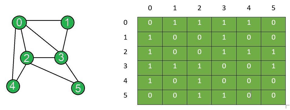
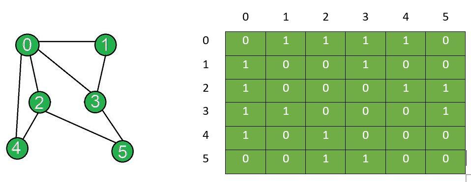
Input: N = 6, Edges[] = {{0, 1}, {0, 2}, {0, 3}, {0, 4}, {1, 3}, {2, 3}, {2, 4}, {2, 5}, {3, 5}}, X = 2, Y = 3
Output:
Adjacency matrix after edge insertion:
0 1 1 1 1 0
1 0 0 1 0 0
1 0 0 1 1 1
1 1 1 0 0 1
1 0 1 0 0 0
0 0 1 1 0 0
Adjacency matrix after edge removal:
0 1 1 1 1 0
1 0 0 1 0 0
1 0 0 0 1 1
1 1 0 0 0 1
1 0 1 0 0 0
0 0 1 1 0 0
Explanation:
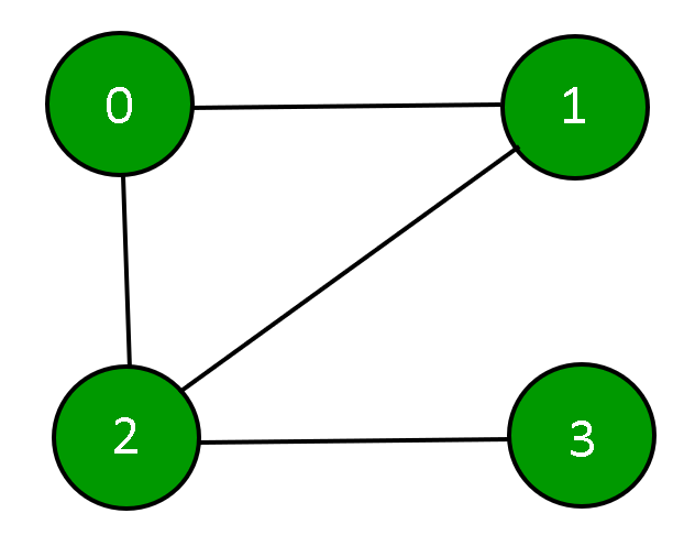
The graph and the corresponding adjacency matrix after insertion of edges:
The graph after removal and adjacency matrix after removal of edge between vertex X and Y:
Input: N = 6, Edges[] = {{0, 1}, {0, 2}, {0, 3}, {0, 4}, {1, 3}, {2, 3}, {2, 4}, {2, 5}, {3, 5}}, X = 3, Y = 5
Output:
Adjacency matrix after edge insertion:
0 1 1 1 1 0
1 0 0 1 0 0
1 0 0 1 1 1
1 1 1 0 0 1
1 0 1 0 0 0
0 0 1 1 0 0
Adjacency matrix after edge removal:
0 1 1 1 1 0
1 0 0 1 0 0
1 0 0 1 1 1
1 1 1 0 0 0
1 0 1 0 0 0
0 0 1 0 0 0
Approach:
Initialize a matrix of dimensions N x N and follow the steps below:
- Inserting an edge: To insert an edge between two vertices suppose i and j, set the corresponding values in the adjacency matrix equal to 1, i.e. g[i][j]=1 and g[j][i]=1 if both the vertices i and j exists.
- Removing an edge: To remove an edge between two vertices suppose i and j, set the corresponding values in the adjacency matrix equal to 0. That is, set g[i][j]=0 and g[j][i]=0 if both the vertices i and j exists.
Below is the implementation of the above approach:
C++
#include <iostream>
using namespace std;
class Graph {
private:
int n;
int g[10][10];
public:
Graph(int x)
{
n = x;
for (int i = 0; i < n; i++) {
for (int j = 0; j < n; j++) {
g[i][j] = 0;
}
}
}
void displayAdjacencyMatrix()
{
for (int i = 0; i < n; i++) {
cout << "\n";
for (int j = 0; j < n; j++) {
cout << " " << g[i][j];
}
}
}
void addEdge(int x, int y)
{
if ((x < 0) || (x >= n)) {
cout << "Vertex" << x
<< " does not exist!";
}
if ((y < 0) || (y >= n)) {
cout << "Vertex" << y
<< " does not exist!";
}
if (x == y) {
cout << "Same Vertex!";
}
else {
g[y][x] = 1;
g[x][y] = 1;
}
}
void removeEdge(int x, int y)
{
if ((x < 0) || (x >= n)) {
cout << "Vertex" << x
<< " does not exist!";
}
if ((y < 0) || (y >= n)) {
cout << "Vertex" << y
<< " does not exist!";
}
if (x == y) {
cout << "Same Vertex!";
}
else {
g[y][x] = 0;
g[x][y] = 0;
}
}
};
int main()
{
int N = 6, X = 2, Y = 3;
Graph obj(N);
obj.addEdge(0, 1);
obj.addEdge(0, 2);
obj.addEdge(0, 3);
obj.addEdge(0, 4);
obj.addEdge(1, 3);
obj.addEdge(2, 3);
obj.addEdge(2, 4);
obj.addEdge(2, 5);
obj.addEdge(3, 5);
cout << "Adjacency matrix after"
<< " edge insertions:\n";
obj.displayAdjacencyMatrix();
obj.removeEdge(X, Y);
cout << "\nAdjacency matrix after"
<< " edge removal:\n";
obj.displayAdjacencyMatrix();
return 0;
}
|
Java
class Graph {
private int n;
private int[][] g = new int[10][10];
Graph(int x)
{
this.n = x;
for (int i = 0; i < n; ++i) {
for (int j = 0; j < n; ++j) {
g[i][j] = 0;
}
}
}
public void displayAdjacencyMatrix()
{
for (int i = 0; i < n; ++i) {
System.out.println();
for (int j = 0; j < n; ++j) {
System.out.print(" " + g[i][j]);
}
}
System.out.println();
}
public void addEdge(int x, int y)
{
if ((x < 0) || (x >= n)) {
System.out.printf("Vertex " + x
+ " does not exist!");
}
if ((y < 0) || (y >= n)) {
System.out.printf("Vertex " + y
+ " does not exist!");
}
if (x == y) {
System.out.println("Same Vertex!");
}
else {
g[y][x] = 1;
g[x][y] = 1;
}
}
public void removeEdge(int x, int y)
{
if ((x < 0) || (x >= n)) {
System.out.printf("Vertex " + x
+ " does not exist!");
}
if ((y < 0) || (y >= n)) {
System.out.printf("Vertex " + y
+ " does not exist!");
}
if (x == y) {
System.out.println("Same Vertex!");
}
else {
g[y][x] = 0;
g[x][y] = 0;
}
}
}
class Main {
public static void main(String[] args)
{
int N = 6, X = 2, Y = 3;
Graph obj = new Graph(N);
obj.addEdge(0, 1);
obj.addEdge(0, 2);
obj.addEdge(0, 3);
obj.addEdge(0, 4);
obj.addEdge(1, 3);
obj.addEdge(2, 3);
obj.addEdge(2, 4);
obj.addEdge(2, 5);
obj.addEdge(3, 5);
System.out.println("Adjacency matrix after"
+ " edge insertions:");
obj.displayAdjacencyMatrix();
obj.removeEdge(2, 3);
System.out.println("\nAdjacency matrix after"
+ " edge removal:");
obj.displayAdjacencyMatrix();
}
}
|
Python3
class Graph:
__n = 0
__g = [[0 for x in range(10)]
for y in range(10)]
def __init__(self, x):
self.__n = x
for i in range(0, self.__n):
for j in range(0, self.__n):
self.__g[i][j] = 0
def displayAdjacencyMatrix(self):
for i in range(0, self.__n):
print()
for j in range(0, self.__n):
print("", self.__g[i][j], end = "")
def addEdge(self, x, y):
if (x < 0) or (x >= self.__n):
print("Vertex {} does not exist!".format(x))
if (y < 0) or (y >= self.__n):
print("Vertex {} does not exist!".format(y))
if(x == y):
print("Same Vertex!")
else:
self.__g[y][x] = 1
self.__g[x][y] = 1
def removeEdge(self, x, y):
if (x < 0) or (x >= self.__n):
print("Vertex {} does not exist!".format(x))
if (y < 0) or (y >= self.__n):
print("Vertex {} does not exist!".format(y))
if(x == y):
print("Same Vertex!")
else:
self.__g[y][x] = 0
self.__g[x][y] = 0
obj = Graph(6);
obj.addEdge(0, 1)
obj.addEdge(0, 2)
obj.addEdge(0, 3)
obj.addEdge(0, 4)
obj.addEdge(1, 3)
obj.addEdge(2, 3)
obj.addEdge(2, 4)
obj.addEdge(2, 5)
obj.addEdge(3, 5)
print("Adjacency matrix after "
"edge insertions:\n")
obj.displayAdjacencyMatrix();
obj.removeEdge(2, 3);
print("\nAdjacency matrix after "
"edge removal:\n")
obj.displayAdjacencyMatrix();
|
C#
using System;
class Graph{
private int n;
private int[,] g = new int[10, 10];
public Graph(int x)
{
this.n = x;
for(int i = 0; i < n; ++i)
{
for(int j = 0; j < n; ++j)
{
g[i, j] = 0;
}
}
}
public void displayAdjacencyMatrix()
{
for(int i = 0; i < n; ++i)
{
Console.WriteLine();
for(int j = 0; j < n; ++j)
{
Console.Write(" " + g[i, j]);
}
}
}
public void addEdge(int x, int y)
{
if ((x < 0) || (x >= n))
{
Console.WriteLine("Vertex {0} does " +
"not exist!", x);
}
if ((y < 0) || (y >= n))
{
Console.WriteLine("Vertex {0} does " +
"not exist!", y);
}
if (x == y)
{
Console.WriteLine("Same Vertex!");
}
else
{
g[y, x] = 1;
g[x, y] = 1;
}
}
public void removeEdge(int x, int y)
{
if ((x < 0) || (x >= n))
{
Console.WriteLine("Vertex {0} does" +
"not exist!", x);
}
if ((y < 0) || (y >= n))
{
Console.WriteLine("Vertex {0} does" +
"not exist!", y);
}
if (x == y)
{
Console.WriteLine("Same Vertex!");
}
else
{
g[y, x] = 0;
g[x, y] = 0;
}
}
}
class GFG{
public static void Main(String[] args)
{
Graph obj = new Graph(6);
obj.addEdge(0, 1);
obj.addEdge(0, 2);
obj.addEdge(0, 3);
obj.addEdge(0, 4);
obj.addEdge(1, 3);
obj.addEdge(2, 3);
obj.addEdge(2, 4);
obj.addEdge(2, 5);
obj.addEdge(3, 5);
Console.WriteLine("Adjacency matrix after " +
"edge insertions:\n");
obj.displayAdjacencyMatrix();
obj.removeEdge(2, 3);
Console.WriteLine("\nAdjacency matrix after " +
"edge removal:");
obj.displayAdjacencyMatrix();
}
}
|
Javascript
<script>
var n = 0;
var g = Array.from(Array(10), ()=>Array(10).fill(0));
function initialize(x)
{
n = x;
for(var i = 0; i < n; ++i)
{
for(var j = 0; j < n; ++j)
{
g[i][j] = 0;
}
}
}
function displayAdjacencyMatrix()
{
for(var i = 0; i < n; ++i)
{
document.write("<br>");
for(var j = 0; j < n; ++j)
{
document.write(" " + g[i][j]);
}
}
}
function addEdge(x, y)
{
if ((x < 0) || (x >= n))
{
document.write(`Vertex ${x} does not exist!`);
}
if ((y < 0) || (y >= n))
{
document.write(`Vertex ${y} does not exist!`);
}
if (x == y)
{
document.write("Same Vertex!<br>");
}
else
{
g[y][x] = 1;
g[x][y] = 1;
}
}
function removeEdge(x, y)
{
if ((x < 0) || (x >= n))
{
document.write(`Vertex ${x} does not exist!`);
}
if ((y < 0) || (y >= n))
{
document.write(`Vertex ${y} does not exist!`);
}
if (x == y)
{
document.write("Same Vertex!<br>");
}
else
{
g[y][x] = 0;
g[x][y] = 0;
}
}
initialize(6);
addEdge(0, 1);
addEdge(0, 2);
addEdge(0, 3);
addEdge(0, 4);
addEdge(1, 3);
addEdge(2, 3);
addEdge(2, 4);
addEdge(2, 5);
addEdge(3, 5);
document.write("Adjacency matrix after " +
"edge insertions:<br>");
displayAdjacencyMatrix();
removeEdge(2, 3);
document.write("<br>Adjacency matrix after " +
"edge removal:<br>");
displayAdjacencyMatrix();
</script>
|
Output:
Adjacency matrix after edge insertions:

 0 1 1 1 1 0
 1 0 0 1 0 0
 1 0 0 1 1 1
 1 1 1 0 0 1
 1 0 1 0 0 0
 0 0 1 1 0 0
Adjacency matrix after edge removal:

 0 1 1 1 1 0
 1 0 0 1 0 0
 1 0 0 0 1 1
 1 1 0 0 0 1
 1 0 1 0 0 0
 0 0 1 1 0 0
Time Complexity: Insertion and Deletion of an edge requires O(1) complexity while it takes O(N2) to display the adjacency matrix.
Auxiliary Space: O(N2)
------
Applications, Advantages and Disadvantages of Graph
Graph is a non-linear data structure that contains nodes (vertices) and edges. A graph is a collection of set of vertices and edges (formed by connecting two vertices). A graph is defined as G = {V, E} where V is the set of vertices and E is the set of edges.
Graphs can be used to model a wide variety of real-world problems, including social networks, transportation networks, and communication networks. They can be represented in various ways, such as by a set of vertices and a set of edges, or by a matrix or an adjacency list. The two most common types of graphs are directed and undirected graphs.
Terminologies of Graphs:
.An edge is one of the two primary units used to form graphs. Each edge has two ends, which are vertices to which it is attached.
.If two vertices are endpoints of the same edge, they are adjacent.
.A vertex’s outgoing edges are directed edges that point to the origin.
.A vertex’s incoming edges are directed edges that point to the vertex’s destination.
.The total number of edges occurring to a vertex in a graph is its degree.
.A vertex with an in-degree of zero is referred to as a source vertex, while one with an out-degree of zero is known as sink vertex.
.A path is a set of alternating vertices and edges, with each vertex connected by an edge.
.The path that starts and finishes at the same vertex is known as a cycle.
.A path with unique vertices is called a simple path.
.A spanning subgraph that is also a tree is known as a spanning tree.
.A connected component is the unconnected graph’s most connected subgraph.
.A bridge, which is an edge of removal, would sever the graph.
.Forest is a graph without a cycle.
Graph Representation:
Graph can be represented in the following ways:
- Set Representation: Set representation of a graph involves two sets: Set of vertices V = {V1, V2, V3, V4} and set of edges E = {{V1, V2}, {V2, V3}, {V3, V4}, {V4, V1}}. This representation is efficient for memory but does not allow parallel edges.
- Sequential Representation: This representation of a graph can be represented by means of matrices: Adjacency Matrix, Incidence matrix and Path matrix.
- Adjacency Matrix: This matrix includes information about the adjacent nodes. Here, aij = 1 if there is an edge from Vi to Vj otherwise 0. It is a matrix of order V×V.
- Incidence Matrix: This matrix includes information about the incidence of edges on the nodes. Here, aij = 1 if the jth edge Ej is incident on ith vertex Vi otherwise 0. It is a matrix of order V×E.
- Path Matrix: This matrix includes information about the simple path between two vertices. Here, Pij = 1 if there is a path from Vi to Vj otherwise 0. It is also called as reachability matrix of graph G.
- Linked Representation: This representation gives the information about the nodes to which a specific node is connected i.e. adjacency lists. This representation gives the adjacency lists of the vertices with the help of array and linked lists. In the adjacency lists, the vertices which are connected with the specific vertex are arranged in the form of lists which is connected to that vertex.
Real-Time Applications of Graph:
- Social media analysis: Social media platforms generate vast amounts of data in real-time, which can be analyzed using graphs to identify trends, sentiment, and key influencers. This can be useful for marketing, customer service, and reputation management.
- Network monitoring: Graphs can be used to monitor network traffic in real-time, allowing network administrators to identify potential bottlenecks, security threats, and other issues. This is critical for ensuring the smooth operation of complex networks.
- Financial trading: Graphs can be used to analyze real-time financial data, such as stock prices and market trends, to identify patterns and make trading decisions. This is particularly important for high-frequency trading, where even small delays can have a significant impact on profits.
- Internet of Things (IoT) management: IoT devices generate vast amounts of data in real-time, which can be analyzed using graphs to identify patterns, optimize performance, and detect anomalies. This is important for managing large-scale IoT deployments.
- Autonomous vehicles: Graphs can be used to model the real-time environment around autonomous vehicles, allowing them to navigate safely and efficiently. This requires real-time data from sensors and other sources, which can be processed using graph algorithms.
- Disease surveillance: Graphs can be used to model the spread of infectious diseases in real-time, allowing health officials to identify outbreaks and implement effective containment strategies. This is particularly important during pandemics or other public health emergencies.
- The best example of graphs in the real world is Facebook. Each person on Facebook is a node and is connected through edges. Thus, A is a friend of B. B is a friend of C, and so on.
Advantages of Graph:
- Representing complex data: Graphs are effective tools for representing complex data, especially when the relationships between the data points are not straightforward. They can help to uncover patterns, trends, and insights that may be difficult to see using other methods.
- Efficient data processing: Graphs can be processed efficiently using graph algorithms, which are specifically designed to work with graph data structures. This makes it possible to perform complex operations on large datasets quickly and effectively.
- Network analysis: Graphs are commonly used in network analysis to study relationships between individuals or organizations, as well as to identify important nodes and edges in a network. This is useful in a variety of fields, including social sciences, business, and marketing.
- Pathfinding: Graphs can be used to find the shortest path between two points, which is a common problem in computer science, logistics, and transportation planning.
- Visualization: Graphs are highly visual, making it easy to communicate complex data and relationships in a clear and concise way. This makes them useful for presentations, reports, and data analysis.
- Machine learning: Graphs can be used in machine learning to model complex relationships between variables, such as in recommendation systems or fraud detection.
- Graphs are used in computer science to depict the flow of computation.
- Users on Facebook are referred to as vertices, and if they are friends, there is an edge connecting them. The Friend Suggestion system on Facebook is based on graph theory.
- You come across the Resources Allocation Graph in the Operating System, where each process and resource are regarded vertically. Edges are drawn from resources to assigned functions or from the requesting process to the desired resources. A stalemate will develop if this results in the establishment of a cycle.
- Web pages are referred to as vertices on the World Wide Web. Suppose there is a link from page A to page B that can represent an edge. this application is an illustration of a directed graph.
- Graph transformation systems manipulate graphs in memory using rules, Graph databases store and query graph-structured data in a transaction-safe, perment manner.
Disadvantages of Graph:
- Limited representation: Graphs can only represent relationships between objects, and not their properties or attributes. This means that in order to fully understand the data, it may be necessary to supplement the graph with additional information.
- Difficulty in interpretation: Graphs can be difficult to interpret, especially if they are large or complex. This can make it challenging to extract meaningful insights from the data, and may require advanced analytical techniques or domain expertise.
- Scalability issues: As the number of nodes and edges in a graph increases, the processing time and memory required to analyze it also increases. This can make it difficult to work with large or complex graphs.
- Data quality issues: Graphs are only as good as the data they are based on, and if the data is incomplete, inconsistent, or inaccurate, the graph may not accurately reflect the relationships between objects.
- Lack of standardization: There are many different types of graphs, and each has its own strengths and weaknesses. This can make it difficult to compare graphs from different sources, or to choose the best type of graph for a given analysis.
- Privacy concerns: Graphs can reveal sensitive information about individuals or organizations, which can raise privacy concerns, especially in social network analysis or marketing.
------
Transitive Closure of a Graph using DFS
Given a directed graph, find out if a vertex v is reachable from another vertex u for all vertex pairs (u, v) in the given graph. Here reachable means that there is a path from vertex u to v. The reach-ability matrix is called transitive closure of a graph.
For example, consider below graph:
.png)
Graph
Transitive closure of above graphs is
1 1 1 1
1 1 1 1
1 1 1 1
0 0 0 1
We have discussed an O(V3) solution for this here. The solution was based on Floyd Warshall Algorithm. In this post, DFS solution is discussed. So for dense graph, it would become O(V3) and for sparse graph, it would become O(V2).
Below are the abstract steps of the algorithm.
- Create a matrix tc[V][V] that would finally have transitive closure of the given graph. Initialize all entries of tc[][] as 0.
- Call DFS for every node of the graph to mark reachable vertices in tc[][]. In recursive calls to DFS, we don’t call DFS for an adjacent vertex if it is already marked as reachable in tc[][].
- Below is the implementation of the above idea. The code uses adjacency list representation of input graph and builds a matrix tc[V][V] such that tc[u][v] would be true if v is reachable from u.
Implementation:
// C++ program to print transitive closure of a graph
#include <bits/stdc++.h>
using namespace std;

class Graph {
    int V; // No. of vertices
    bool** tc; // To store transitive closure
    list<int>* adj; // array of adjacency lists
    void DFSUtil(int u, int v);

public:
    Graph(int V); // Constructor

    // function to add an edge to graph
    void addEdge(int v, int w) { adj[v].push_back(w); }

    // prints transitive closure matrix
    void transitiveClosure();
};

Graph::Graph(int V)
{
    this->V = V;
    adj = new list<int>[V];

    tc = new bool*[V];
    for (int i = 0; i < V; i++) {
        tc[i] = new bool[V];
        memset(tc[i], false, V * sizeof(bool));
    }
}

// A recursive DFS traversal function that finds
// all reachable vertices for s.
void Graph::DFSUtil(int s, int v) {
    // Mark reachability from s to v as true.
    tc[s][v] = true;

    // Explore all vertices adjacent to v
    for (int u : adj[v]) {
        // If s is not yet connected to u, explore further
        if (!tc[s][u]) {
            DFSUtil(s, u);
        }
    }
}
// The function to find transitive closure. It uses
// recursive DFSUtil()
void Graph::transitiveClosure()
{
    // Call the recursive helper function to print DFS
    // traversal starting from all vertices one by one
    for (int i = 0; i < V; i++)
        DFSUtil(i,
                i); // Every vertex is reachable from self.

    for (int i = 0; i < V; i++) {
        for (int j = 0; j < V; j++)
            cout << tc[i][j] << " ";
        cout << endl;
    }
}

// Driver code
int main()
{

    // Create a graph given in the above diagram
    Graph g(4);
    g.addEdge(0, 1);
    g.addEdge(0, 2);
    g.addEdge(1, 2);
    g.addEdge(2, 0);
    g.addEdge(2, 3);
    g.addEdge(3, 3);
    cout << "Transitive closure matrix is \n";
    g.transitiveClosure();
    return 0;
}
// JAVA program to print transitive
// closure of a graph.

import java.util.ArrayList;
import java.util.Arrays;

// A directed graph using
// adjacency list representation
public class Graph {

        // No. of vertices in graph
    private int vertices;

        // adjacency list
    private ArrayList<Integer>[] adjList;

        // To store transitive closure
    private int[][] tc;

    // Constructor
    public Graph(int vertices) {

             // initialise vertex count
             this.vertices = vertices;
             this.tc = new int[this.vertices][this.vertices];

             // initialise adjacency list
             initAdjList();
    }

    // utility method to initialise adjacency list
    @SuppressWarnings("unchecked")
    private void initAdjList() {

        adjList = new ArrayList[vertices];
        for (int i = 0; i < vertices; i++) {
            adjList[i] = new ArrayList<>();
        }
    }

    // add edge from u to v
    public void addEdge(int u, int v) {

      // Add v to u's list.
        adjList[u].add(v);
    }

    // The function to find transitive
    // closure. It uses
    // recursive DFSUtil()
    public void transitiveClosure() {

        // Call the recursive helper
        // function to print DFS
        // traversal starting from all
        // vertices one by one
        for (int i = 0; i < vertices; i++) {
            dfsUtil(i, i);
        }

        for (int i = 0; i < vertices; i++) {
          System.out.println(Arrays.toString(tc[i]));
        }
    }

    // A recursive DFS traversal
    // function that finds
    // all reachable vertices for s
    private void dfsUtil(int s, int v) {

        // Mark reachability from
        // s to v as true.
       if(s==v){
          tc[s][v] = 1;
       }
      else
        tc[s][v] = 1;

        // Find all the vertices reachable
        // through v
        for (int adj : adjList[v]) {
            if (tc[s][adj]==0) {
                dfsUtil(s, adj);
            }
        }
    }

    // Driver Code
    public static void main(String[] args) {

        // Create a graph given
        // in the above diagram
        Graph g = new Graph(4);

        g.addEdge(0, 1);
        g.addEdge(0, 2);
        g.addEdge(1, 2);
        g.addEdge(2, 0);
        g.addEdge(2, 3);
        g.addEdge(3, 3);
        System.out.println("Transitive closure " +
                "matrix is");

        g.transitiveClosure();

    }
}


// This code is contributed
// by Himanshu Shekhar
OutputTransitive closure matrix is
1 1 1 1
1 1 1 1
1 1 1 1
0 0 0 1
Time Complexity : O(V^3) where V is the number of vertexes . For dense graph, it would become O(V3) and for sparse graph, it would become O(V2).
Auxiliary Space: O(V^2) where V is number of vertices.
------
Floyd Warshall Algorithm
The Floyd-Warshall algorithm, named after its creators Robert Floyd and Stephen Warshall, is a fundamental algorithm in computer science and graph theory. It is used to find the shortest paths between all pairs of nodes in a weighted graph. This algorithm is highly efficient and can handle graphs with both positive and negative edge weights, making it a versatile tool for solving a wide range of network and connectivity problems.

Floyd Warshall Algorithm:
The Floyd Warshall Algorithm is an all pair shortest path algorithm unlike Dijkstra and Bellman Ford which are single source shortest path algorithms. This algorithm works for both the directed and undirected weighted graphs. But, it does not work for the graphs with negative cycles (where the sum of the edges in a cycle is negative). It follows Dynamic Programming approach to check every possible path going via every possible node in order to calculate shortest distance between every pair of nodes.
Idea Behind Floyd Warshall Algorithm:
Suppose we have a graph G[][] with V vertices from 1 to N. Now we have to evaluate a shortestPathMatrix[][] where shortestPathMatrix[i][j] represents the shortest path between vertices i and j.
Obviously the shortest path between i to j will have some k number of intermediate nodes. The idea behind floyd warshall algorithm is to treat each and every vertex from 1 to N as an intermediate node one by one.
The following figure shows the above optimal substructure property in floyd warshall algorithm:
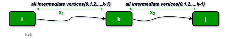
Floyd Warshall Algorithm Algorithm:
- Initialize the solution matrix same as the input graph matrix as a first step.
- Then update the solution matrix by considering all vertices as an intermediate vertex.
- The idea is to pick all vertices one by one and updates all shortest paths which include the picked vertex as an intermediate vertex in the shortest path.
- When we pick vertex number k as an intermediate vertex, we already have considered vertices {0, 1, 2, .. k-1} as intermediate vertices.
- For every pair (i, j) of the source and destination vertices respectively, there are two possible cases.
- k is not an intermediate vertex in shortest path from i to j. We keep the value of dist[i][j] as it is.
- k is an intermediate vertex in shortest path from i to j. We update the value of dist[i][j] as dist[i][k] + dist[k][j], if dist[i][j] > dist[i][k] + dist[k][j]
Pseudo-Code of Floyd Warshall Algorithm :
For k = 0 to n – 1
For i = 0 to n – 1
For j = 0 to n – 1
Distance[i, j] = min(Distance[i, j], Distance[i, k] + Distance[k, j])
where i = source Node, j = Destination Node, k = Intermediate Node
Illustration of Floyd Warshall Algorithm :
Suppose we have a graph as shown in the image:
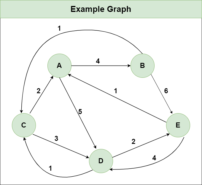
Step 1: Initialize the Distance[][] matrix using the input graph such that Distance[i][j]= weight of edge from i to j, also Distance[i][j] = Infinity if there is no edge from i to j.
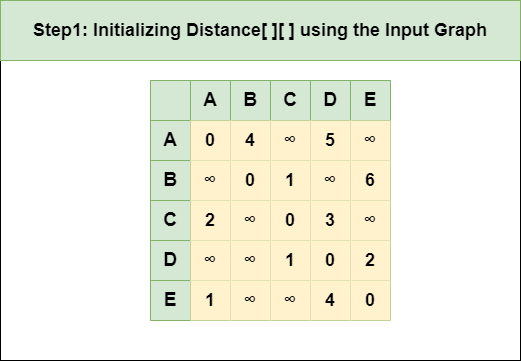
Step 2: Treat node A as an intermediate node and calculate the Distance[][] for every {i,j} node pair using the formula:
= Distance[i][j] = minimum (Distance[i][j], (Distance from i to A) + (Distance from A to j ))
= Distance[i][j] = minimum (Distance[i][j], Distance[i][A] + Distance[A][j])
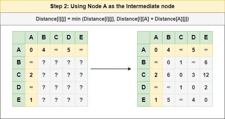
Step 3: Treat node B as an intermediate node and calculate the Distance[][] for every {i,j} node pair using the formula:
= Distance[i][j] = minimum (Distance[i][j], (Distance from i to B) + (Distance from B to j ))
= Distance[i][j] = minimum (Distance[i][j], Distance[i][B] + Distance[B][j])
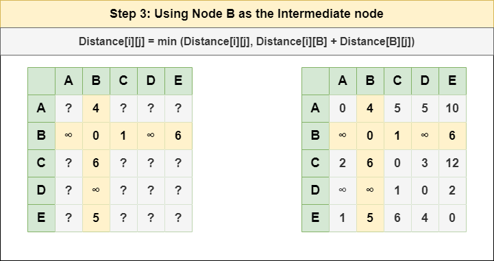
Step 4: Treat node C as an intermediate node and calculate the Distance[][] for every {i,j} node pair using the formula:
= Distance[i][j] = minimum (Distance[i][j], (Distance from i to C) + (Distance from C to j ))
= Distance[i][j] = minimum (Distance[i][j], Distance[i][C] + Distance[C][j])
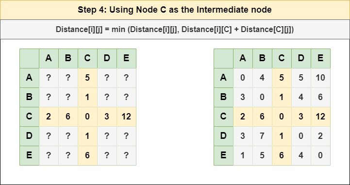
Step 5: Treat node D as an intermediate node and calculate the Distance[][] for every {i,j} node pair using the formula:
= Distance[i][j] = minimum (Distance[i][j], (Distance from i to D) + (Distance from D to j ))
= Distance[i][j] = minimum (Distance[i][j], Distance[i][D] + Distance[D][j])
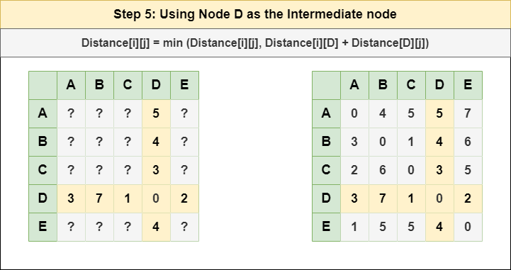
Step 6: Treat node E as an intermediate node and calculate the Distance[][] for every {i,j} node pair using the formula:
= Distance[i][j] = minimum (Distance[i][j], (Distance from i to E) + (Distance from E to j ))
= Distance[i][j] = minimum (Distance[i][j], Distance[i][E] + Distance[E][j])
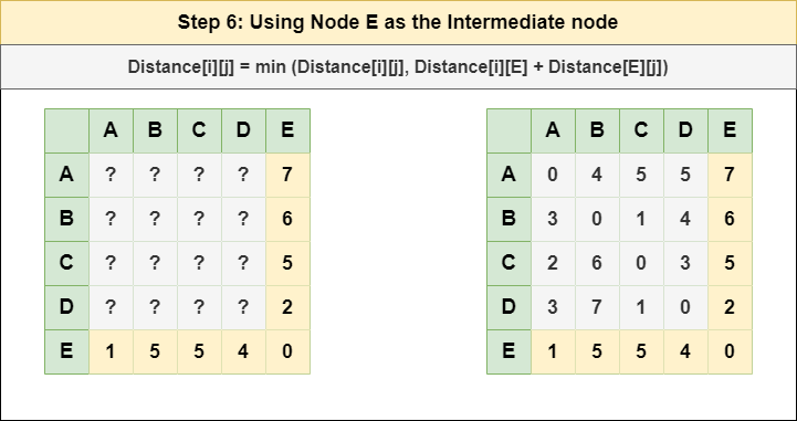
Step 7: Since all the nodes have been treated as an intermediate node, we can now return the updated Distance[][] matrix as our answer matrix.
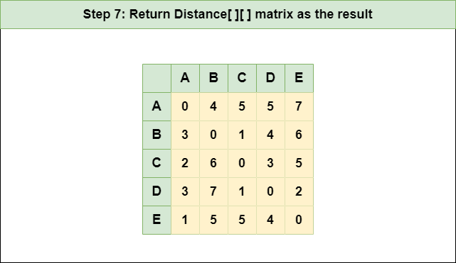
Below is the implementation of the above approach:
// C++ Program for Floyd Warshall Algorithm
#include <bits/stdc++.h>
using namespace std;

// Number of vertices in the graph
#define V 4

/* Define Infinite as a large enough
value.This value will be used for
vertices not connected to each other */
#define INF 99999

// A function to print the solution matrix
void printSolution(int dist[][V]);

// Solves the all-pairs shortest path
// problem using Floyd Warshall algorithm
void floydWarshall(int dist[][V])
{

    int i, j, k;

    /* Add all vertices one by one to
    the set of intermediate vertices.
    ---> Before start of an iteration,
    we have shortest distances between all
    pairs of vertices such that the
    shortest distances consider only the
    vertices in set {0, 1, 2, .. k-1} as
    intermediate vertices.
    ----> After the end of an iteration,
    vertex no. k is added to the set of
    intermediate vertices and the set becomes {0, 1, 2, ..
    k} */
    for (k = 0; k < V; k++) {
        // Pick all vertices as source one by one
        for (i = 0; i < V; i++) {
            // Pick all vertices as destination for the
            // above picked source
            for (j = 0; j < V; j++) {
                // If vertex k is on the shortest path from
                // i to j, then update the value of
                // dist[i][j]
                if (dist[i][j] > (dist[i][k] + dist[k][j])
                    && (dist[k][j] != INF
                        && dist[i][k] != INF))
                    dist[i][j] = dist[i][k] + dist[k][j];
            }
        }
    }

    // Print the shortest distance matrix
    printSolution(dist);
}

/* A utility function to print solution */
void printSolution(int dist[][V])
{
    cout << "The following matrix shows the shortest "
            "distances"
            " between every pair of vertices \n";
    for (int i = 0; i < V; i++) {
        for (int j = 0; j < V; j++) {
            if (dist[i][j] == INF)
                cout << "INF"
                     << " ";
            else
                cout << dist[i][j] << "   ";
        }
        cout << endl;
    }
}

// Driver's code
int main()
{
    /* Let us create the following weighted graph
            10
    (0)------->(3)
        |     /|\
    5 |     |
        |     | 1
    \|/     |
    (1)------->(2)
            3     */
    int graph[V][V] = { { 0, 5, INF, 10 },
                        { INF, 0, 3, INF },
                        { INF, INF, 0, 1 },
                        { INF, INF, INF, 0 } };

    // Function call
    floydWarshall(graph);
    return 0;
}

// This code is contributed by Mythri J L
// Java program for Floyd Warshall All Pairs Shortest
// Path algorithm.
import java.io.*;
import java.lang.*;
import java.util.*;

class AllPairShortestPath {
    final static int INF = 99999, V = 4;

    void floydWarshall(int dist[][])
    {

        int i, j, k;

        /* Add all vertices one by one
           to the set of intermediate
           vertices.
          ---> Before start of an iteration,
               we have shortest
               distances between all pairs
               of vertices such that
               the shortest distances consider
               only the vertices in
               set {0, 1, 2, .. k-1} as
               intermediate vertices.
          ----> After the end of an iteration,
                vertex no. k is added
                to the set of intermediate
                vertices and the set
                becomes {0, 1, 2, .. k} */
        for (k = 0; k < V; k++) {
            // Pick all vertices as source one by one
            for (i = 0; i < V; i++) {
                // Pick all vertices as destination for the
                // above picked source
                for (j = 0; j < V; j++) {
                    // If vertex k is on the shortest path
                    // from i to j, then update the value of
                    // dist[i][j]
                    if (dist[i][k] + dist[k][j]
                        < dist[i][j])
                        dist[i][j]
                            = dist[i][k] + dist[k][j];
                }
            }
        }

        // Print the shortest distance matrix
        printSolution(dist);
    }

    void printSolution(int dist[][])
    {
        System.out.println(
            "The following matrix shows the shortest "
            + "distances between every pair of vertices");
        for (int i = 0; i < V; ++i) {
            for (int j = 0; j < V; ++j) {
                if (dist[i][j] == INF)
                    System.out.print("INF ");
                else
                    System.out.print(dist[i][j] + "   ");
            }
            System.out.println();
        }
    }

    // Driver's code
    public static void main(String[] args)
    {
        /* Let us create the following weighted graph
           10
        (0)------->(3)
        |         /|\
        5 |          |
        |          | 1
        \|/         |
        (1)------->(2)
           3           */
        int graph[][] = { { 0, 5, INF, 10 },
                          { INF, 0, 3, INF },
                          { INF, INF, 0, 1 },
                          { INF, INF, INF, 0 } };
        AllPairShortestPath a = new AllPairShortestPath();

        // Function call
        a.floydWarshall(graph);
    }
}

// Contributed by Aakash Hasija
OutputThe following matrix shows the shortest distances between every pair of vertices
0 5 8 9
INF 0 3 4
INF INF 0 1
INF INF INF 0
- Time Complexity: O(V3), where V is the number of vertices in the graph and we run three nested loops each of size V
- Auxiliary Space: O(V2), to create a 2-D matrix in order to store the shortest distance for each pair of nodes.
Note: The above program only prints the shortest distances. We can modify the solution to print the shortest paths also by storing the predecessor information in a separate 2D matrix.
Why Floyd-Warshall Algorithm better for Dense Graphs and not for Sparse Graphs?
Dense Graph: A graph in which the number of edges are significantly much higher than the number of vertices.
Sparse Graph: A graph in which the number of edges are very much low.
No matter how many edges are there in the graph the Floyd Warshall Algorithm runs for O(V3) times therefore it is best suited for Dense graphs. In the case of sparse graphs, Johnson’s Algorithm is more suitable.
Real World Applications of Floyd-Warshall Algorithm:
- In computer networking, the algorithm can be used to find the shortest path between all pairs of nodes in a network. This is termed as network routing.
- Flight Connectivity In the aviation industry to find the shortest path between the airports.
- GIS(Geographic Information Systems) applications often involve analyzing spatial data, such as road networks, to find the shortest paths between locations.
- Kleene’s algorithm which is a generalization of floyd warshall, can be used to find regular expression for a regular language.
------
How to find Shortest Paths from Source to all Vertices using Dijkstra’s Algorithm
Given a weighted graph and a source vertex in the graph, find the shortest paths from the source to all the other vertices in the given graph.
Note: The given graph does not contain any negative edge.
Examples:
Input: src = 0, the graph is shown below.
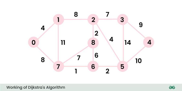
Output: 0 4 12 19 21 11 9 8 14
Explanation: The distance from 0 to 1 = 4.
The minimum distance from 0 to 2 = 12. 0->1->2
The minimum distance from 0 to 3 = 19. 0->1->2->3
The minimum distance from 0 to 4 = 21. 0->7->6->5->4
The minimum distance from 0 to 5 = 11. 0->7->6->5
The minimum distance from 0 to 6 = 9. 0->7->6
The minimum distance from 0 to 7 = 8. 0->7
The minimum distance from 0 to 8 = 14. 0->1->2->8
The idea is to generate a SPT (shortest path tree) with a given source as a root. Maintain an Adjacency Matrix with two sets,
- one set contains vertices included in the shortest-path tree,
- other set includes vertices not yet included in the shortest-path tree.
At every step of the algorithm, find a vertex that is in the other set (set not yet included) and has a minimum distance from the source.
Algorithm:
- Create a set sptSet (shortest path tree set) that keeps track of vertices included in the shortest path tree, i.e., whose minimum distance from the source is calculated and finalized. Initially, this set is empty.
- Assign a distance value to all vertices in the input graph. Initialize all distance values as INFINITE. Assign the distance value as 0 for the source vertex so that it is picked first.
- While sptSet doesn’t include all vertices
- Pick a vertex u that is not there in sptSet and has a minimum distance value.
- Include u to sptSet.
- Then update the distance value of all adjacent vertices of u.
- To update the distance values, iterate through all adjacent vertices.
- For every adjacent vertex v, if the sum of the distance value of u (from source) and weight of edge u-v, is less than the distance value of v, then update the distance value of v.
Note: We use a boolean array sptSet[] to represent the set of vertices included in SPT. If a value sptSet[v] is true, then vertex v is included in SPT, otherwise not. Array dist[] is used to store the shortest distance values of all vertices.
Illustration of Dijkstra Algorithm:
To understand the Dijkstra’s Algorithm lets take a graph and find the shortest path from source to all nodes.
Consider below graph and src = 0
Step 1:
- The set sptSet is initially empty and distances assigned to vertices are {0, INF, INF, INF, INF, INF, INF, INF} where INF indicates infinite.
- Now pick the vertex with a minimum distance value. The vertex 0 is picked, include it in sptSet. So sptSet becomes {0}. After including 0 to sptSet, update distance values of its adjacent vertices.
- Adjacent vertices of 0 are 1 and 7. The distance values of 1 and 7 are updated as 4 and 8.
The following subgraph shows vertices and their distance values, only the vertices with finite distance values are shown. The vertices included in SPT are shown in green colour.
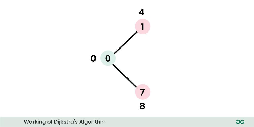
Step 2:
- Pick the vertex with minimum distance value and not already included in SPT (not in sptSET). The vertex 1 is picked and added to sptSet.
- So sptSet now becomes {0, 1}. Update the distance values of adjacent vertices of 1.
- The distance value of vertex 2 becomes 12.
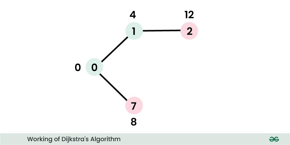
Step 3:
- Pick the vertex with minimum distance value and not already included in SPT (not in sptSET). Vertex 7 is picked. So sptSet now becomes {0, 1, 7}.
- Update the distance values of adjacent vertices of 7. The distance value of vertex 6 and 8 becomes finite (15 and 9 respectively).
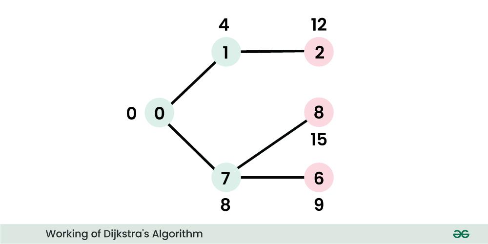
Step 4:
- Pick the vertex with minimum distance value and not already included in SPT (not in sptSET). Vertex 6 is picked. So sptSet now becomes {0, 1, 7, 6}.
- Update the distance values of adjacent vertices of 6. The distance value of vertex 5 and 8 are updated.
.jpg)
We repeat the above steps until sptSet includes all vertices of the given graph. Finally, we get the following Shortest Path Tree (SPT).
.jpg)
Below is the implementation of the above approach:
// C++ program for Dijkstra's single source shortest path
// algorithm. The program is for adjacency matrix
// representation of the graph
#include <iostream>
using namespace std;
#include <limits.h>

// Number of vertices in the graph
#define V 9

// A utility function to find the vertex with minimum
// distance value, from the set of vertices not yet included
// in shortest path tree
int minDistance(int dist[], bool sptSet[])
{

    // Initialize min value
    int min = INT_MAX, min_index;

    for (int v = 0; v < V; v++)
        if (sptSet[v] == false && dist[v] <= min)
            min = dist[v], min_index = v;

    return min_index;
}

// A utility function to print the constructed distance
// array
void printSolution(int dist[])
{
    cout << "Vertex \t Distance from Source" << endl;
    for (int i = 0; i < V; i++)
        cout << i << " \t\t\t\t" << dist[i] << endl;
}

// Function that implements Dijkstra's single source
// shortest path algorithm for a graph represented using
// adjacency matrix representation
void dijkstra(int graph[V][V], int src)
{
    int dist[V]; // The output array.  dist[i] will hold the
                 // shortest
    // distance from src to i

    bool sptSet[V]; // sptSet[i] will be true if vertex i is
                    // included in shortest
    // path tree or shortest distance from src to i is
    // finalized

    // Initialize all distances as INFINITE and stpSet[] as
    // false
    for (int i = 0; i < V; i++)
        dist[i] = INT_MAX, sptSet[i] = false;

    // Distance of source vertex from itself is always 0
    dist[src] = 0;

    // Find shortest path for all vertices
    for (int count = 0; count < V - 1; count++) {
        // Pick the minimum distance vertex from the set of
        // vertices not yet processed. u is always equal to
        // src in the first iteration.
        int u = minDistance(dist, sptSet);

        // Mark the picked vertex as processed
        sptSet[u] = true;

        // Update dist value of the adjacent vertices of the
        // picked vertex.
        for (int v = 0; v < V; v++)

            // Update dist[v] only if is not in sptSet,
            // there is an edge from u to v, and total
            // weight of path from src to  v through u is
            // smaller than current value of dist[v]
            if (!sptSet[v] && graph[u][v]
                && dist[u] != INT_MAX
                && dist[u] + graph[u][v] < dist[v])
                dist[v] = dist[u] + graph[u][v];
    }

    // print the constructed distance array
    printSolution(dist);
}

// driver's code
int main()
{

    /* Let us create the example graph discussed above */
    int graph[V][V] = { { 0, 4, 0, 0, 0, 0, 0, 8, 0 },
                        { 4, 0, 8, 0, 0, 0, 0, 11, 0 },
                        { 0, 8, 0, 7, 0, 4, 0, 0, 2 },
                        { 0, 0, 7, 0, 9, 14, 0, 0, 0 },
                        { 0, 0, 0, 9, 0, 10, 0, 0, 0 },
                        { 0, 0, 4, 14, 10, 0, 2, 0, 0 },
                        { 0, 0, 0, 0, 0, 2, 0, 1, 6 },
                        { 8, 11, 0, 0, 0, 0, 1, 0, 7 },
                        { 0, 0, 2, 0, 0, 0, 6, 7, 0 } };

    // Function call
    dijkstra(graph, 0);

    return 0;
}

// This code is contributed by shivanisinghss2110
// A Java program for Dijkstra's single source shortest path
// algorithm. The program is for adjacency matrix
// representation of the graph
import java.io.*;
import java.lang.*;
import java.util.*;

class ShortestPath {
    // A utility function to find the vertex with minimum
    // distance value, from the set of vertices not yet
    // included in shortest path tree
    static final int V = 9;
    int minDistance(int dist[], Boolean sptSet[])
    {
        // Initialize min value
        int min = Integer.MAX_VALUE, min_index = -1;

        for (int v = 0; v < V; v++)
            if (sptSet[v] == false && dist[v] <= min) {
                min = dist[v];
                min_index = v;
            }

        return min_index;
    }

    // A utility function to print the constructed distance
    // array
    void printSolution(int dist[])
    {
        System.out.println(
            "Vertex \t\t Distance from Source");
        for (int i = 0; i < V; i++)
            System.out.println(i + " \t\t " + dist[i]);
    }

    // Function that implements Dijkstra's single source
    // shortest path algorithm for a graph represented using
    // adjacency matrix representation
    void dijkstra(int graph[][], int src)
    {
        int dist[] = new int[V]; // The output array.
                                 // dist[i] will hold
        // the shortest distance from src to i

        // sptSet[i] will true if vertex i is included in
        // shortest path tree or shortest distance from src
        // to i is finalized
        Boolean sptSet[] = new Boolean[V];

        // Initialize all distances as INFINITE and stpSet[]
        // as false
        for (int i = 0; i < V; i++) {
            dist[i] = Integer.MAX_VALUE;
            sptSet[i] = false;
        }

        // Distance of source vertex from itself is always 0
        dist[src] = 0;

        // Find shortest path for all vertices
        for (int count = 0; count < V - 1; count++) {
            // Pick the minimum distance vertex from the set
            // of vertices not yet processed. u is always
            // equal to src in first iteration.
            int u = minDistance(dist, sptSet);

            // Mark the picked vertex as processed
            sptSet[u] = true;

            // Update dist value of the adjacent vertices of
            // the picked vertex.
            for (int v = 0; v < V; v++)

                // Update dist[v] only if is not in sptSet,
                // there is an edge from u to v, and total
                // weight of path from src to v through u is
                // smaller than current value of dist[v]
                if (!sptSet[v] && graph[u][v] != 0
                    && dist[u] != Integer.MAX_VALUE
                    && dist[u] + graph[u][v] < dist[v])
                    dist[v] = dist[u] + graph[u][v];
        }

        // print the constructed distance array
        printSolution(dist);
    }

    // Driver's code
    public static void main(String[] args)
    {
        /* Let us create the example graph discussed above
         */
        int graph[][]
            = new int[][] { { 0, 4, 0, 0, 0, 0, 0, 8, 0 },
                            { 4, 0, 8, 0, 0, 0, 0, 11, 0 },
                            { 0, 8, 0, 7, 0, 4, 0, 0, 2 },
                            { 0, 0, 7, 0, 9, 14, 0, 0, 0 },
                            { 0, 0, 0, 9, 0, 10, 0, 0, 0 },
                            { 0, 0, 4, 14, 10, 0, 2, 0, 0 },
                            { 0, 0, 0, 0, 0, 2, 0, 1, 6 },
                            { 8, 11, 0, 0, 0, 0, 1, 0, 7 },
                            { 0, 0, 2, 0, 0, 0, 6, 7, 0 } };
        ShortestPath t = new ShortestPath();

        // Function call
        t.dijkstra(graph, 0);
    }
}
// This code is contributed by Aakash Hasija
OutputVertex Distance from Source
0 0
1 4
2 12
3 19
4 21
5 11
6 9
7 8
8 14
Time Complexity: O(V2)
Auxiliary Space: O(V)
Notes:
- The code calculates the shortest distance but doesn’t calculate the path information. Create a parent array, update the parent array when distance is updated and use it to show the shortest path from source to different vertices.
- The time Complexity of the implementation is O(V2). If the input graph is represented using adjacency list, it can be reduced to O(E * log V) with the help of a binary heap. Please see Dijkstra’s Algorithm for Adjacency List Representation for more details.
- Dijkstra’s algorithm doesn’t work for graphs with negative weight cycles.
Why Dijkstra’s Algorithms fails for the Graphs having Negative Edges ?
The problem with negative weights arises from the fact that Dijkstra’s algorithm assumes that once a node is added to the set of visited nodes, its distance is finalized and will not change. However, in the presence of negative weights, this assumption can lead to incorrect results.
Consider the following graph for the example:
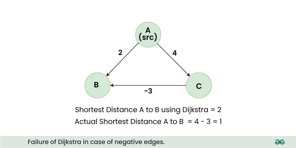
In the above graph, A is the source node, among the edges A to B and A to C , A to B is the smaller weight and Dijkstra assigns the shortest distance of B as 2, but because of existence of a negative edge from C to B, the actual shortest distance reduces to 1 which Dijkstra fails to detect.
Note: We use Bellman Ford’s Shortest path algorithm in case we have negative edges in the graph.
Dijkstra’s Algorithm using Adjacency List in O(E logV):
For Dijkstra’s algorithm, it is always recommended to use Heap (or priority queue) as the required operations (extract minimum and decrease key) match with the speciality of the heap (or priority queue). However, the problem is, that priority_queue doesn’t support the decrease key. To resolve this problem, do not update a key, but insert one more copy of it. So we allow multiple instances of the same vertex in the priority queue. This approach doesn’t require decreasing key operations and has below important properties.
- Whenever the distance of a vertex is reduced, we add one more instance of a vertex in priority_queue. Even if there are multiple instances, we only consider the instance with minimum distance and ignore other instances.
- The time complexity remains O(E * LogV) as there will be at most O(E) vertices in the priority queue and O(logE) is the same as O(logV)
Below is the implementation of the above approach:
// C++ Program to find Dijkstra's shortest path using
// priority_queue in STL
#include <bits/stdc++.h>
using namespace std;
#define INF 0x3f3f3f3f

// iPair ==> Integer Pair
typedef pair<int, int> iPair;

// This class represents a directed graph using
// adjacency list representation
class Graph {
    int V; // No. of vertices

    // In a weighted graph, we need to store vertex
    // and weight pair for every edge
    list<pair<int, int> >* adj;

public:
    Graph(int V); // Constructor

    // function to add an edge to graph
    void addEdge(int u, int v, int w);

    // prints shortest path from s
    void shortestPath(int s);
};

// Allocates memory for adjacency list
Graph::Graph(int V)
{
    this->V = V;
    adj = new list<iPair>[V];
}

void Graph::addEdge(int u, int v, int w)
{
    adj[u].push_back(make_pair(v, w));
    adj[v].push_back(make_pair(u, w));
}

// Prints shortest paths from src to all other vertices
void Graph::shortestPath(int src)
{
    // Create a priority queue to store vertices that
    // are being preprocessed. This is weird syntax in C++.
    // Refer below link for details of this syntax
    // https://www.geeksforgeeks.org/implement-min-heap-using-stl/
    priority_queue<iPair, vector<iPair>, greater<iPair> >
        pq;

    // Create a vector for distances and initialize all
    // distances as infinite (INF)
    vector<int> dist(V, INF);

    // Insert source itself in priority queue and initialize
    // its distance as 0.
    pq.push(make_pair(0, src));
    dist[src] = 0;

    /* Looping till priority queue becomes empty (or all
    distances are not finalized) */
    while (!pq.empty()) {
        // The first vertex in pair is the minimum distance
        // vertex, extract it from priority queue.
        // vertex label is stored in second of pair (it
        // has to be done this way to keep the vertices
        // sorted distance (distance must be first item
        // in pair)
        int u = pq.top().second;
        pq.pop();

        // 'i' is used to get all adjacent vertices of a
        // vertex
        list<pair<int, int> >::iterator i;
        for (i = adj[u].begin(); i != adj[u].end(); ++i) {
            // Get vertex label and weight of current
            // adjacent of u.
            int v = (*i).first;
            int weight = (*i).second;

            // If there is shorted path to v through u.
            if (dist[v] > dist[u] + weight) {
                // Updating distance of v
                dist[v] = dist[u] + weight;
                pq.push(make_pair(dist[v], v));
            }
        }
    }

    // Print shortest distances stored in dist[]
    printf("Vertex Distance from Source\n");
    for (int i = 0; i < V; ++i)
        printf("%d \t\t %d\n", i, dist[i]);
}

// Driver's code
int main()
{
    // create the graph given in above figure
    int V = 9;
    Graph g(V);

    // making above shown graph
    g.addEdge(0, 1, 4);
    g.addEdge(0, 7, 8);
    g.addEdge(1, 2, 8);
    g.addEdge(1, 7, 11);
    g.addEdge(2, 3, 7);
    g.addEdge(2, 8, 2);
    g.addEdge(2, 5, 4);
    g.addEdge(3, 4, 9);
    g.addEdge(3, 5, 14);
    g.addEdge(4, 5, 10);
    g.addEdge(5, 6, 2);
    g.addEdge(6, 7, 1);
    g.addEdge(6, 8, 6);
    g.addEdge(7, 8, 7);

    // Function call
    g.shortestPath(0);

    return 0;
}
import java.util.*;

class Graph {
    private int V;
    private List<List<iPair>> adj;

    Graph(int V) {
        this.V = V;
        adj = new ArrayList<>();
        for (int i = 0; i < V; i++) {
            adj.add(new ArrayList<>());
        }
    }

    void addEdge(int u, int v, int w) {
        adj.get(u).add(new iPair(v, w));
        adj.get(v).add(new iPair(u, w));
    }

    void shortestPath(int src) {
        PriorityQueue<iPair> pq = new PriorityQueue<>(V, Comparator.comparingInt(o -> o.first));
        int[] dist = new int[V];
        Arrays.fill(dist, Integer.MAX_VALUE);

        pq.add(new iPair(0, src));
        dist[src] = 0;

        while (!pq.isEmpty()) {
            int u = pq.poll().second;

            for (iPair v : adj.get(u)) {
                if (dist[v.first] > dist[u] + v.second) {
                    dist[v.first] = dist[u] + v.second;
                    pq.add(new iPair(dist[v.first], v.first));
                }
            }
        }

        System.out.println("Vertex Distance from Source");
        for (int i = 0; i < V; i++) {
            System.out.println(i + "\t\t" + dist[i]);
        }
    }

    static class iPair {
        int first, second;

        iPair(int first, int second) {
            this.first = first;
            this.second = second;
        }
    }
}

public class Main {
    public static void main(String[] args) {
        int V = 9;
        Graph g = new Graph(V);

        g.addEdge(0, 1, 4);
        g.addEdge(0, 7, 8);
        g.addEdge(1, 2, 8);
        g.addEdge(1, 7, 11);
        g.addEdge(2, 3, 7);
        g.addEdge(2, 8, 2);
        g.addEdge(2, 5, 4);
        g.addEdge(3, 4, 9);
        g.addEdge(3, 5, 14);
        g.addEdge(4, 5, 10);
        g.addEdge(5, 6, 2);
        g.addEdge(6, 7, 1);
        g.addEdge(6, 8, 6);
        g.addEdge(7, 8, 7);

        g.shortestPath(0);
    }
}
OutputVertex Distance from Source
0 0
1 4
2 12
3 19
4 21
5 11
6 9
7 8
8 14
Time Complexity: O(E * logV), Where E is the number of edges and V is the number of vertices.
Auxiliary Space: O(V)
Applications of Dijkstra’s Algorithm:
- Google maps uses Dijkstra algorithm to show shortest distance between source and destination.
- In computer networking, Dijkstra’s algorithm forms the basis for various routing protocols, such as OSPF (Open Shortest Path First) and IS-IS (Intermediate System to Intermediate System).
- Transportation and traffic management systems use Dijkstra’s algorithm to optimize traffic flow, minimize congestion, and plan the most efficient routes for vehicles.
- Airlines use Dijkstra’s algorithm to plan flight paths that minimize fuel consumption, reduce travel time.
- Dijkstra’s algorithm is applied in electronic design automation for routing connections on integrated circuits and very-large-scale integration (VLSI) chips.
For a more detailed explanation refer to this article Dijkstra’s Shortest Path Algorithm using priority_queue of STL.
------
Breadth First Search or BFS for a Graph
Breadth First Search (BFS) is a fundamental graph traversal algorithm. It involves visiting all the connected nodes of a graph in a level-by-level manner. In this article, we will look into the concept of BFS and how it can be applied to graphs effectively
Breadth First Search (BFS) for a Graph:
Breadth First Search (BFS) is a graph traversal algorithm that explores all the vertices in a graph at the current depth before moving on to the vertices at the next depth level. It starts at a specified vertex and visits all its neighbors before moving on to the next level of neighbors. BFS is commonly used in algorithms for pathfinding, connected components, and shortest path problems in graphs.
Relation between BFS for Graph and BFS for Tree:
Breadth-First Traversal (BFS) for a graph is similar to the Breadth-First Traversal of a tree.
The only catch here is, that, unlike trees, graphs may contain cycles, so we may come to the same node again. To avoid processing a node more than once, we divide the vertices into two categories:
A boolean visited array is used to mark the visited vertices. For simplicity, it is assumed that all vertices are reachable from the starting vertex. BFS uses a queue data structure for traversal.
Breadth First Search (BFS) for a Graph Algorithm:
Let’s discuss the algorithm for the BFS:
- Initialization: Enqueue the starting node into a queue and mark it as visited.
- Exploration: While the queue is not empty:
- Dequeue a node from the queue and visit it (e.g., print its value).
- For each unvisited neighbor of the dequeued node:
- Enqueue the neighbor into the queue.
- Mark the neighbor as visited.
- Termination: Repeat step 2 until the queue is empty.
This algorithm ensures that all nodes in the graph are visited in a breadth-first manner, starting from the starting node.
How Does the BFS Algorithm Work?
Starting from the root, all the nodes at a particular level are visited first and then the nodes of the next level are traversed till all the nodes are visited.
To do this a queue is used. All the adjacent unvisited nodes of the current level are pushed into the queue and the nodes of the current level are marked visited and popped from the queue.
Illustration:
Let us understand the working of the algorithm with the help of the following example.
Step1: Initially queue and visited arrays are empty.
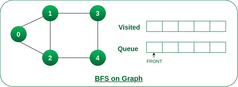
Queue and visited arrays are empty initially.
Step2: Push node 0 into queue and mark it visited.
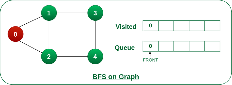
Push node 0 into queue and mark it visited.
Step 3: Remove node 0 from the front of queue and visit the unvisited neighbours and push them into queue.
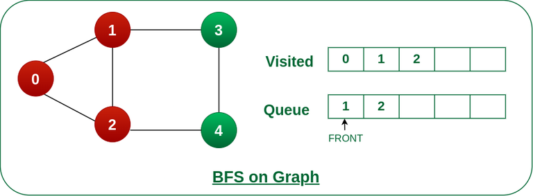
Remove node 0 from the front of queue and visited the unvisited neighbours and push into queue.
Step 4: Remove node 1 from the front of queue and visit the unvisited neighbours and push them into queue.
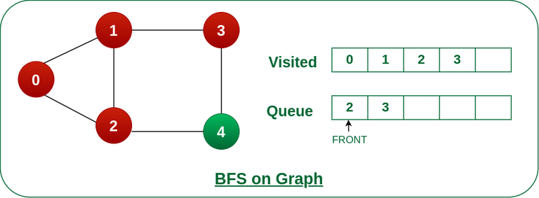
Remove node 1 from the front of queue and visited the unvisited neighbours and push
Step 5: Remove node 2 from the front of queue and visit the unvisited neighbours and push them into queue.

Remove node 2 from the front of queue and visit the unvisited neighbours and push them into queue.
Step 6: Remove node 3 from the front of queue and visit the unvisited neighbours and push them into queue.
As we can see that every neighbours of node 3 is visited, so move to the next node that are in the front of the queue.

Remove node 3 from the front of queue and visit the unvisited neighbours and push them into queue.
Steps 7: Remove node 4 from the front of queue and visit the unvisited neighbours and push them into queue.
As we can see that every neighbours of node 4 are visited, so move to the next node that is in the front of the queue.
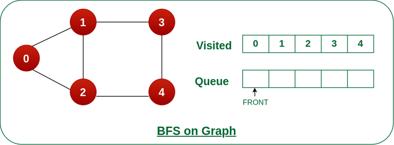
Remove node 4 from the front of queue and visit the unvisited neighbours and push them into queue.
Now, Queue becomes empty, So, terminate these process of iteration.
Implementation of BFS for Graph using Adjacency List:
#include <iostream>
#include <queue>
#include <vector>

using namespace std;

// Function to perform Breadth First Search on a graph
// represented using adjacency list
void bfs(vector<vector<int> >& adjList, int startNode,
         vector<bool>& visited)
{
    // Create a queue for BFS
    queue<int> q;

    // Mark the current node as visited and enqueue it
    visited[startNode] = true;
    q.push(startNode);

    // Iterate over the queue
    while (!q.empty()) {
        // Dequeue a vertex from queue and print it
        int currentNode = q.front();
        q.pop();
        cout << currentNode << " ";

        // Get all adjacent vertices of the dequeued vertex
        // currentNode If an adjacent has not been visited,
        // then mark it visited and enqueue it
        for (int neighbor : adjList[currentNode]) {
            if (!visited[neighbor]) {
                visited[neighbor] = true;
                q.push(neighbor);
            }
        }
    }
}

// Function to add an edge to the graph
void addEdge(vector<vector<int> >& adjList, int u, int v)
{
    adjList[u].push_back(v);
}

int main()
{
    // Number of vertices in the graph
    int vertices = 5;

    // Adjacency list representation of the graph
    vector<vector<int> > adjList(vertices);

    // Add edges to the graph
    addEdge(adjList, 0, 1);
    addEdge(adjList, 0, 2);
    addEdge(adjList, 1, 3);
    addEdge(adjList, 1, 4);
    addEdge(adjList, 2, 4);

    // Mark all the vertices as not visited
    vector<bool> visited(vertices, false);

    // Perform BFS traversal starting from vertex 0
    cout << "Breadth First Traversal starting from vertex "
            "0: ";
    bfs(adjList, 0, visited);

    return 0;
}
import java.util.LinkedList;
import java.util.Queue;

// Class to represent a graph using adjacency list
class Graph {
    int vertices;
    LinkedList<Integer>[] adjList;

    @SuppressWarnings("unchecked") Graph(int vertices)
    {
        this.vertices = vertices;
        adjList = new LinkedList[vertices];
        for (int i = 0; i < vertices; ++i)
            adjList[i] = new LinkedList<>();
    }

    // Function to add an edge to the graph
    void addEdge(int u, int v) { adjList[u].add(v); }

    // Function to perform Breadth First Search on a graph
    // represented using adjacency list
    void bfs(int startNode)
    {
        // Create a queue for BFS
        Queue<Integer> queue = new LinkedList<>();
        boolean[] visited = new boolean[vertices];

        // Mark the current node as visited and enqueue it
        visited[startNode] = true;
        queue.add(startNode);

        // Iterate over the queue
        while (!queue.isEmpty()) {
            // Dequeue a vertex from queue and print it
            int currentNode = queue.poll();
            System.out.print(currentNode + " ");

            // Get all adjacent vertices of the dequeued
            // vertex currentNode If an adjacent has not
            // been visited, then mark it visited and
            // enqueue it
            for (int neighbor : adjList[currentNode]) {
                if (!visited[neighbor]) {
                    visited[neighbor] = true;
                    queue.add(neighbor);
                }
            }
        }
    }
}

public class Main {
    public static void main(String[] args)
    {
        // Number of vertices in the graph
        int vertices = 5;

        // Create a graph
        Graph graph = new Graph(vertices);

        // Add edges to the graph
        graph.addEdge(0, 1);
        graph.addEdge(0, 2);
        graph.addEdge(1, 3);
        graph.addEdge(1, 4);
        graph.addEdge(2, 4);

        // Perform BFS traversal starting from vertex 0
        System.out.print(
            "Breadth First Traversal starting from vertex 0: ");
        graph.bfs(0);
    }
}
OutputBreadth First Traversal starting from vertex 0: 0 1 2 3 4
Time Complexity: O(V+E), where V is the number of nodes and E is the number of edges.
Auxiliary Space: O(V)
Complexity Analysis of Breadth-First Search (BFS) Algorithm:
Time Complexity of BFS Algorithm: O(V + E)
- BFS explores all the vertices and edges in the graph. In the worst case, it visits every vertex and edge once. Therefore, the time complexity of BFS is O(V + E), where V and E are the number of vertices and edges in the given graph.
Space Complexity of BFS Algorithm: O(V)
- BFS uses a queue to keep track of the vertices that need to be visited. In the worst case, the queue can contain all the vertices in the graph. Therefore, the space complexity of BFS is O(V), where V and E are the number of vertices and edges in the given graph.
Applications of BFS in Graphs:
BFS has various applications in graph theory and computer science, including:
- Shortest Path Finding: BFS can be used to find the shortest path between two nodes in an unweighted graph. By keeping track of the parent of each node during the traversal, the shortest path can be reconstructed.
- Cycle Detection: BFS can be used to detect cycles in a graph. If a node is visited twice during the traversal, it indicates the presence of a cycle.
- Connected Components: BFS can be used to identify connected components in a graph. Each connected component is a set of nodes that can be reached from each other.
- Topological Sorting: BFS can be used to perform topological sorting on a directed acyclic graph (DAG). Topological sorting arranges the nodes in a linear order such that for any edge (u, v), u appears before v in the order.
- Level Order Traversal of Binary Trees: BFS can be used to perform a level order traversal of a binary tree. This traversal visits all nodes at the same level before moving to the next level.
- Network Routing: BFS can be used to find the shortest path between two nodes in a network, making it useful for routing data packets in network protocols.
Problems on Breadth First Search or BFS for a Graph:
FAQs on Breadth First Search (BFS) for a Graph:
Question 1: What is BFS and how does it work?
Answer: BFS is a graph traversal algorithm that systematically explores a graph by visiting all the vertices at a given level before moving on to the next level. It starts from a starting vertex, enqueues it into a queue, and marks it as visited. Then, it dequeues a vertex from the queue, visits it, and enqueues all its unvisited neighbors into the queue. This process continues until the queue is empty.
Question 2: What are the applications of BFS?
Answer: BFS has various applications, including finding the shortest path in an unweighted graph, detecting cycles in a graph, topologically sorting a directed acyclic graph (DAG), finding connected components in a graph, and solving puzzles like mazes and Sudoku.
Question 3: What is the time complexity of BFS?
Answer: The time complexity of BFS is O(V + E), where V is the number of vertices and E is the number of edges in the graph.
Question 4: What is the space complexity of BFS?
Answer: The space complexity of BFS is O(V), as it uses a queue to keep track of the vertices that need to be visited.
Question 5: What are the advantages of using BFS?
Answer: BFS is simple to implement and efficient for finding the shortest path in an unweighted graph. It also guarantees that all the vertices in the graph are visited.
Related Articles:
------
Applications, Advantages and Disadvantages of Breadth First Search (BFS)
We have earlier discussed Breadth First Traversal Algorithm for Graphs. Here in this article, we will see the applications, advantages, and disadvantages of the Breadth First Search.
Applications of Breadth First Search:
1. Shortest Path and Minimum Spanning Tree for unweighted graph: In an unweighted graph, the shortest path is the path with the least number of edges. With Breadth First, we always reach a vertex from a given source using the minimum number of edges. Also, in the case of unweighted graphs, any spanning tree is Minimum Spanning Tree and we can use either Depth or Breadth first traversal for finding a spanning tree.
2. Minimum Spanning Tree for weighted graphs: We can also find Minimum Spanning Tree for weighted graphs using BFT, but the condition is that the weight should be non-negative and the same for each pair of vertices.
3. Peer-to-Peer Networks: In Peer-to-Peer Networks like BitTorrent, Breadth First Search is used to find all neighbor nodes.
4. Crawlers in Search Engines: Crawlers build an index using Breadth First. The idea is to start from the source page and follow all links from the source and keep doing the same. Depth First Traversal can also be used for crawlers, but the advantage of Breadth First Traversal is, the depth or levels of the built tree can be limited.
5. Social Networking Websites: In social networks, we can find people within a given distance ‘k’ from a person using Breadth First Search till ‘k’ levels.
6. GPS Navigation systems: Breadth First Search is used to find all neighboring locations.
7. Broadcasting in Network: In networks, a broadcasted packet follows Breadth First Search to reach all nodes.
8. In Garbage Collection: Breadth First Search is used in copying garbage collection using Cheney’s algorithm. Breadth First Search is preferred over Depth First Search because of a better locality of reference.
9. Cycle detection in undirected graph: In undirected graphs, either Breadth First Search or Depth First Search can be used to detect a cycle. We can use BFS to detect cycle in a directed graph also.
10. Ford–Fulkerson algorithm In Ford – Fulkerson algorithm, we can either use Breadth First or Depth First Traversal to find the maximum flow. Breadth First Traversal is preferred as it reduces the worst-case time complexity to O(VE2).
11. To test if a graph is Bipartite: We can either use Breadth First or Depth First Traversal.
12. Path Finding: We can either use Breadth First or Depth First Traversal to find if there is a path between two vertices.
13. Finding all nodes within one connected component: We can either use Breadth First or Depth First Traversal to find all nodes reachable from a given node.
14. AI: In AI, BFS is used in traversing a game tree to find the best move.
15. Network Security: In the field of network security, BFS is used in traversing a network to find all the devices connected to it.
16. Connected Component: We can find all connected components in an undirected graph.
17. Topological sorting: BFS can be used to find a topological ordering of the nodes in a directed acyclic graph (DAG).
18. Image processing: BFS can be used to flood-fill an image with a particular color or to find connected components of pixels.
19. Recommender systems: BFS can be used to find similar items in a large dataset by traversing the items’ connections in a similarity graph.
20. Other usages: Many algorithms like Prim’s Minimum Spanning Tree and Dijkstra’s Single Source Shortest Path use structures similar to Breadth First Search.
Advantages of Breadth First Search:
- BFS will never get trapped exploring the useful path forever.
- If there is a solution, BFS will definitely find it.
- If there is more than one solution then BFS can find the minimal one that requires less number of steps.
- Low storage requirement – linear with depth.
- Easily programmable.
Disadvantages of Breadth First Search:
The main drawback of BFS is its memory requirement. Since each level of the graph must be saved in order to generate the next level and the amount of memory is proportional to the number of nodes stored the space complexity of BFS is O(bd ), where b is the branching factor(the number of children at each node, the outdegree) and d is the depth. As a result, BFS is severely space-bound in practice so will exhaust the memory available on typical computers in a matter of minutes.
------
Depth First Search or DFS for a Graph
Depth First Traversal (or DFS) for a graph is similar to Depth First Traversal of a tree. The only catch here is, that, unlike trees, graphs may contain cycles (a node may be visited twice). To avoid processing a node more than once, use a boolean visited array. A graph can have more than one DFS traversal.
Example:
Input: n = 4, e = 6
0 -> 1, 0 -> 2, 1 -> 2, 2 -> 0, 2 -> 3, 3 -> 3
Output: DFS from vertex 1 : 1 2 0 3
Explanation:
DFS Diagram:
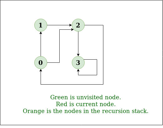
Example 1
Input: n = 4, e = 6
2 -> 0, 0 -> 2, 1 -> 2, 0 -> 1, 3 -> 3, 1 -> 3
Output: DFS from vertex 2 : 2 0 1 3
Explanation:
DFS Diagram:
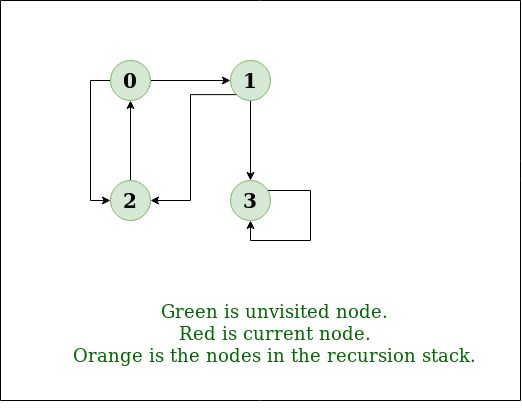
Example 2
How does DFS work?
Depth-first search is an algorithm for traversing or searching tree or graph data structures. The algorithm starts at the root node (selecting some arbitrary node as the root node in the case of a graph) and explores as far as possible along each branch before backtracking.
Let us understand the working of Depth First Search with the help of the following illustration:
Step1: Initially stack and visited arrays are empty.
-copy-660.webp)
Stack and visited arrays are empty initially.
Step 2: Visit 0 and put its adjacent nodes which are not visited yet into the stack.
-copy-660.webp)
Visit node 0 and put its adjacent nodes (1, 2, 3) into the stack
Step 3: Now, Node 1 at the top of the stack, so visit node 1 and pop it from the stack and put all of its adjacent nodes which are not visited in the stack.
-copy-660.webp)
Visit node 1
Step 4: Now, Node 2 at the top of the stack, so visit node 2 and pop it from the stack and put all of its adjacent nodes which are not visited (i.e, 3, 4) in the stack.
-copy-660.webp)
Visit node 2 and put its unvisited adjacent nodes (3, 4) into the stack
Step 5: Now, Node 4 at the top of the stack, so visit node 4 and pop it from the stack and put all of its adjacent nodes which are not visited in the stack.
-copy-660.webp)
Visit node 4
Step 6: Now, Node 3 at the top of the stack, so visit node 3 and pop it from the stack and put all of its adjacent nodes which are not visited in the stack.
-copy-660.webp)
Visit node 3
Now, Stack becomes empty, which means we have visited all the nodes and our DFS traversal ends.
Below is the implementation of the above approach:
C++
#include <bits/stdc++.h>
using namespace std;
class Graph {
public:
map<int, bool> visited;
map<int, list<int> > adj;
void addEdge(int v, int w);
void DFS(int v);
};
void Graph::addEdge(int v, int w)
{
adj[v].push_back(w);
}
void Graph::DFS(int v)
{
visited[v] = true;
cout << v << " ";
list<int>::iterator i;
for (i = adj[v].begin(); i != adj[v].end(); ++i)
if (!visited[*i])
DFS(*i);
}
int main()
{
Graph g;
g.addEdge(0, 1);
g.addEdge(0, 2);
g.addEdge(1, 2);
g.addEdge(2, 0);
g.addEdge(2, 3);
g.addEdge(3, 3);
cout << "Following is Depth First Traversal"
" (starting from vertex 2) \n";
g.DFS(2);
return 0;
}
|
Java
import java.io.*;
import java.util.*;
class Graph {
private int V;
private LinkedList<Integer> adj[];
@SuppressWarnings("unchecked") Graph(int v)
{
V = v;
adj = new LinkedList[v];
for (int i = 0; i < v; ++i)
adj[i] = new LinkedList();
}
void addEdge(int v, int w)
{
adj[v].add(w);
}
void DFSUtil(int v, boolean visited[])
{
visited[v] = true;
System.out.print(v + " ");
Iterator<Integer> i = adj[v].listIterator();
while (i.hasNext()) {
int n = i.next();
if (!visited[n])
DFSUtil(n, visited);
}
}
void DFS(int v)
{
boolean visited[] = new boolean[V];
DFSUtil(v, visited);
}
public static void main(String args[])
{
Graph g = new Graph(4);
g.addEdge(0, 1);
g.addEdge(0, 2);
g.addEdge(1, 2);
g.addEdge(2, 0);
g.addEdge(2, 3);
g.addEdge(3, 3);
System.out.println(
"Following is Depth First Traversal "
+ "(starting from vertex 2)");
g.DFS(2);
}
}
|
Python3
from collections import defaultdict
class Graph:
def __init__(self):
self.graph = defaultdict(list)
def addEdge(self, u, v):
self.graph[u].append(v)
def DFSUtil(self, v, visited):
visited.add(v)
print(v, end=' ')
for neighbour in self.graph[v]:
if neighbour not in visited:
self.DFSUtil(neighbour, visited)
def DFS(self, v):
visited = set()
self.DFSUtil(v, visited)
if __name__ == "__main__":
g = Graph()
g.addEdge(0, 1)
g.addEdge(0, 2)
g.addEdge(1, 2)
g.addEdge(2, 0)
g.addEdge(2, 3)
g.addEdge(3, 3)
print("Following is Depth First Traversal (starting from vertex 2)")
g.DFS(2)
|
C#
using System;
using System.Collections.Generic;
class Graph {
private int V;
private List<int>[] adj;
Graph(int v)
{
V = v;
adj = new List<int>[ v ];
for (int i = 0; i < v; ++i)
adj[i] = new List<int>();
}
void AddEdge(int v, int w)
{
adj[v].Add(w);
}
void DFSUtil(int v, bool[] visited)
{
visited[v] = true;
Console.Write(v + " ");
List<int> vList = adj[v];
foreach(var n in vList)
{
if (!visited[n])
DFSUtil(n, visited);
}
}
void DFS(int v)
{
bool[] visited = new bool[V];
DFSUtil(v, visited);
}
public static void Main(String[] args)
{
Graph g = new Graph(4);
g.AddEdge(0, 1);
g.AddEdge(0, 2);
g.AddEdge(1, 2);
g.AddEdge(2, 0);
g.AddEdge(2, 3);
g.AddEdge(3, 3);
Console.WriteLine(
"Following is Depth First Traversal "
+ "(starting from vertex 2)");
g.DFS(2);
Console.ReadKey();
}
}
|
Javascript
class Graph
{
constructor(v)
{
this.V = v;
this.adj = new Array(v);
for(let i = 0; i < v; i++)
this.adj[i] = [];
}
addEdge(v, w)
{
this.adj[v].push(w);
}
DFSUtil(v, visited)
{
visited[v] = true;
console.log(v + " ");
for(let i of this.adj[v].values())
{
let n = i
if (!visited[n])
this.DFSUtil(n, visited);
}
}
DFS(v)
{
let visited = new Array(this.V);
for(let i = 0; i < this.V; i++)
visited[i] = false;
this.DFSUtil(v, visited);
}
}
g = new Graph(4);
g.addEdge(0, 1);
g.addEdge(0, 2);
g.addEdge(1, 2);
g.addEdge(2, 0);
g.addEdge(2, 3);
g.addEdge(3, 3);
console.log("Following is Depth First Traversal " +
"(starting from vertex 2)");
g.DFS(2);
|
Output
Following is Depth First Traversal (starting from vertex 2)
2 0 1 3
- Time complexity: O(V + E), where V is the number of vertices and E is the number of edges in the graph.
- Auxiliary Space: O(V + E), since an extra visited array of size V is required, And stack size for iterative call to DFS function.
------
Applications, Advantages and Disadvantages of Depth First Search (DFS)
Depth First Search is a widely used algorithm for traversing a graph. Here we have discussed some applications, advantages, and disadvantages of the algorithm.
Applications of Depth First Search:
1. Detecting cycle in a graph: A graph has a cycle if and only if we see a back edge during DFS. So we can run DFS for the graph and check for back edges.
2. Path Finding: We can specialize the DFS algorithm to find a path between two given vertices u and z.
- Call DFS(G, u) with u as the start vertex.
- Use a stack S to keep track of the path between the start vertex and the current vertex.
- As soon as destination vertex z is encountered, return the path as the contents of the stack
3. Topological Sorting: Topological Sorting is mainly used for scheduling jobs from the given dependencies among jobs. In computer science, applications of this type arise in instruction scheduling, ordering of formula cell evaluation when recomputing formula values in spreadsheets, logic synthesis, determining the order of compilation tasks to perform in makefiles, data serialization, and resolving symbol dependencies in linkers.
4. To test if a graph is bipartite: We can augment either BFS or DFS when we first discover a new vertex, color it opposite its parents, and for each other edge, check it doesn’t link two vertices of the same color. The first vertex in any connected component can be red or black.
5. Finding Strongly Connected Components of a graph: A directed graph is called strongly connected if there is a path from each vertex in the graph to every other vertex. (See this for DFS-based algo for finding Strongly Connected Components)
6. Solving puzzles with only one solution: such as mazes. (DFS can be adapted to find all solutions to a maze by only including nodes on the current path in the visited set.).
7. Web crawlers: Depth-first search can be used in the implementation of web crawlers to explore the links on a website.
8. Maze generation: Depth-first search can be used to generate random mazes.
9. Model checking: Depth-first search can be used in model checking, which is the process of checking that a model of a system meets a certain set of properties.
10. Backtracking: Depth-first search can be used in backtracking algorithms.
Advantages of Depth First Search:
- Memory requirement is only linear with respect to the search graph. This is in contrast with breadth-first search which requires more space. The reason is that the algorithm only needs to store a stack of nodes on the path from the root to the current node.
- The time complexity of a depth-first Search to depth d and branching factor b (the number of children at each node, the outdegree) is O(bd) since it generates the same set of nodes as breadth-first search, but simply in a different order. Thus practically depth-first search is time-limited rather than space-limited.
- If depth-first search finds solution without exploring much in a path then the time and space it takes will be very less.
- DFS requires less memory since only the nodes on the current path are stored. By chance DFS may find a solution without examining much of the search space at all.
Disadvantages of Depth First Search:
- The disadvantage of Depth-First Search is that there is a possibility that it may down the left-most path forever. Even a finite graph can generate an infinite solution to this problem is to impose a cutoff depth on the search. Although ideal cutoff is the solution depth d and this value is rarely known in advance of actually solving the problem. If the chosen cutoff depth is less than d, the algorithm will fail to find a solution, whereas if the cutoff depth is greater than d, a large price is paid in execution time, and the first solution found may not be an optimal one.
- Depth-First Search is not guaranteed to find the solution.
- And there is no guarantee to find a minimal solution, if more than one solution.
------
Difference between BFS and DFS
Breadth-First Search (BFS) and Depth-First Search (DFS) are two fundamental algorithms used for traversing or searching graphs and trees. This article covers the basic difference between Breadth-First Search and Depth-First Search.
.png)
Difference between BFS and DFS
BFS, Breadth-First Search, is a vertex-based technique for finding the shortest path in the graph. It uses a Queue data structure that follows first in first out. In BFS, one vertex is selected at a time when it is visited and marked then its adjacent are visited and stored in the queue. It is slower than DFS.
Example:
 Input:
        A
       / \
      B   C
     /   / \
    D   E   F
Output:
A, B, C, D, E, F
DFS, Depth First Search, is an edge-based technique. It uses the Stack data structure and performs two stages, first visited vertices are pushed into the stack, and second if there are no vertices then visited vertices are popped.
Example:
  Input:
        A
       / \
      B   D
     /   / \
    C   E   F
Output:
A, B, C, D, E, F
Difference Between BFS and DFS:
| Parameters |
BFS |
DFS |
| Stands for |
BFS stands for Breadth First Search. |
DFS stands for Depth First Search. |
| Data Structure |
BFS(Breadth First Search) uses Queue data structure for finding the shortest path. |
DFS(Depth First Search) uses Stack data structure. |
| Definition |
BFS is a traversal approach in which we first walk through all nodes on the same level before moving on to the next level. |
DFS is also a traversal approach in which the traverse begins at the root node and proceeds through the nodes as far as possible until we reach the node with no unvisited nearby nodes. |
| Conceptual Difference |
BFS builds the tree level by level. |
DFS builds the tree sub-tree by sub-tree. |
| Approach used |
It works on the concept of FIFO (First In First Out). |
It works on the concept of LIFO (Last In First Out). |
| Suitable for |
BFS is more suitable for searching vertices closer to the given source. |
DFS is more suitable when there are solutions away from source. |
| Applications |
BFS is used in various applications such as bipartite graphs, shortest paths, etc. |
DFS is used in various applications such as acyclic graphs and finding strongly connected components etc. |
Please also see BFS vs DFS for Binary Tree for the differences for a Binary Tree Traversal.
------
What is Minimum Spanning Tree (MST)
A minimum spanning tree (MST) is defined as a spanning tree that has the minimum weight among all the possible spanning trees
A spanning tree is defined as a tree-like subgraph of a connected, undirected graph that includes all the vertices of the graph. Or, to say in Layman’s words, it is a subset of the edges of the graph that forms a tree (acyclic) where every node of the graph is a part of the tree.
The minimum spanning tree has all the properties of a spanning tree with an added constraint of having the minimum possible weights among all possible spanning trees. Like a spanning tree, there can also be many possible MSTs for a graph.
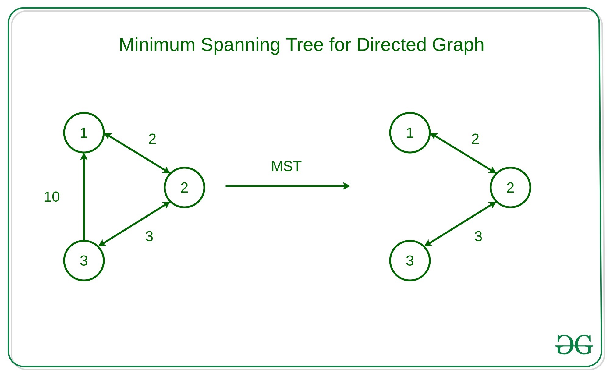
Properties of a Spanning Tree:
The spanning tree holds the below-mentioned principles:
- The number of vertices (V) in the graph and the spanning tree is the same.
- There is a fixed number of edges in the spanning tree which is equal to one less than the total number of vertices ( E = V-1 ).
- The spanning tree should not be disconnected, as in there should only be a single source of component, not more than that.
- The spanning tree should be acyclic, which means there would not be any cycle in the tree.
- The total cost (or weight) of the spanning tree is defined as the sum of the edge weights of all the edges of the spanning tree.
- There can be many possible spanning trees for a graph.
Minimum Spanning Tree:
A minimum spanning tree (MST) is defined as a spanning tree that has the minimum weight among all the possible spanning trees.
The minimum spanning tree has all the properties of a spanning tree with an added constraint of having the minimum possible weights among all possible spanning trees. Like a spanning tree, there can also be many possible MSTs for a graph.
- Let’s look at the MST of the above example Graph,
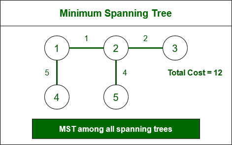
Minimum Spanning Tree
Algorithms to find Minimum Spanning Tree:
There are several algorithms to find the minimum spanning tree from a given graph, some of them are listed below:
Kruskal’s Minimum Spanning Tree Algorithm:
This is one of the popular algorithms for finding the minimum spanning tree from a connected, undirected graph. This is a greedy algorithm. The algorithm workflow is as below:
- First, it sorts all the edges of the graph by their weights,
- Then starts the iterations of finding the spanning tree.
- At each iteration, the algorithm adds the next lowest-weight edge one by one, such that the edges picked until now does not form a cycle.
This algorithm can be implemented efficiently using a DSU ( Disjoint-Set ) data structure to keep track of the connected components of the graph. This is used in a variety of practical applications such as network design, clustering, and data analysis.
Follow the article on “Kruskal’s Minimum Spanning Tree Algorithm” for a better understanding and implementation of the algorithm.
Prim’s Minimum Spanning Tree Algorithm:
This is also a greedy algorithm. This algorithm has the following workflow:
- It starts by selecting an arbitrary vertex and then adding it to the MST.
- Then, it repeatedly checks for the minimum edge weight that connects one vertex of MST to another vertex that is not yet in the MST.
- This process is continued until all the vertices are included in the MST.
To efficiently select the minimum weight edge for each iteration, this algorithm uses priority_queue to store the vertices sorted by their minimum edge weight currently. It also simultaneously keeps track of the MST using an array or other data structure suitable considering the data type it is storing.
This algorithm can be used in various scenarios such as image segmentation based on color, texture, or other features. For Routing, as in finding the shortest path between two points for a delivery truck to follow.
Follow the article on “Prim’s Minimum Spanning Tree Algorithm” for a better understanding and implementation of this algorithm.
Boruvka’s Minimum Spanning Tree Algorithm:
This is also a graph traversal algorithm used to find the minimum spanning tree of a connected, undirected graph. This is one of the oldest algorithms. The algorithm works by iteratively building the minimum spanning tree, starting with each vertex in the graph as its own tree. In each iteration, the algorithm finds the cheapest edge that connects a tree to another tree, and adds that edge to the minimum spanning tree. This is almost similar to the Prim’s algorithm for finding the minimum spanning tree. The algorithm has the following workflow:
- Initialize a forest of trees, with each vertex in the graph as its own tree.
- For each tree in the forest:
- Find the cheapest edge that connects it to another tree. Add these edges to the minimum spanning tree.
- Update the forest by merging the trees connected by the added edges.
- Repeat the above steps until the forest contains only one tree, which is the minimum spanning tree.
The algorithm can be implemented using a data structure such as a priority queue to efficiently find the cheapest edge between trees. Boruvka’s algorithm is a simple and easy-to-implement algorithm for finding minimum spanning trees, but it may not be as efficient as other algorithms for large graphs with many edges.
Follow the article on “Boruvka’s Minimum Spanning Tree Algorithm” for a better understanding and implementation of this algorithm.
To knowing more about the properties and characteristics of Minimum Spanning Tree, click here.
- Network design: Spanning trees can be used in network design to find the minimum number of connections required to connect all nodes. Minimum spanning trees, in particular, can help minimize the cost of the connections by selecting the cheapest edges.
- Image processing: Spanning trees can be used in image processing to identify regions of similar intensity or color, which can be useful for segmentation and classification tasks.
- Biology: Spanning trees and minimum spanning trees can be used in biology to construct phylogenetic trees to represent evolutionary relationships among species or genes.
- Social network analysis: Spanning trees and minimum spanning trees can be used in social network analysis to identify important connections and relationships among individuals or groups.
Some popular interview problems on MST
Some FAQs about Minimum Spanning Trees:
1. Can there be multiple minimum-spanning trees for a given graph?
Yes, a graph can have multiple minimum spanning trees if there are multiple sets of edges with the same minimum total weight.
2. Can Kruskal’s algorithm and Prim’s algorithm be used for directed graphs?
No, Kruskal’s algorithm and Prim’s algorithm are designed for undirected graphs only.
3. Can a disconnected graph have a minimum spanning tree?
No, a disconnected graph cannot have a spanning tree because it does not span all the vertices. Therefore, it also cannot have a minimum spanning tree.
4. Can a minimum spanning tree be found using Dijkstra’s algorithm?
No, Dijkstra’s algorithm is used to find the shortest path between two vertices in a weighted graph. It is not designed to find a minimum spanning tree.
5. What is the time complexity of Kruskal’s and Prim’s algorithms?
Both Kruskal’s and Prim’s algorithms have a time complexity of O(ElogE), where E is the number of edges in the graph.
------